0. Abstract
While the Transformer architecture has become the de-facto standard for natural language processing tasks, its applications to computer vision remain limited. In vision, attention is either applied in conjunction with convolutional networks, or used to replace certain components of convolutional networks while keeping their overall structure in place. We show that this reliance on CNNs is not necessary and a pure transformer applied directly to sequences of image patches can perform very well on image classification tasks. When pre-trained on large amounts of data and transferred to multiple mid-sized or small image recognition benchmarks (ImageNet, CIFAR-100, VTAB, etc.), Vision Transformer (ViT) attains excellent results compared to state-of-the-art convolutional networks while requiring substantially fewer computational resources to train.1
Transformer 아키텍처는 자연어 처리 작업에서 사실상의 표준이 되었지만, 컴퓨터 비전에 대한 적용은 제한적입니다. 비전에서는 어텐션(Attention)이 합성곱 신경망(CNN)과 함께 적용되거나, 합성곱 신경망의 일부 구성 요소를 대체하는 데 사용되지만, 전반적인 구조는 유지됩니다. 우리는 CNN에 대한 의존성이 필요하지 않으며, 이미지 패치(sequence of image patches)에 직접 적용된 순수한 Transformer가 이미지 분류 작업에서 매우 우수한 성능을 발휘할 수 있다는 것을 보여줍니다. 대규모 데이터로 사전 훈련되고 여러 중간 규모 또는 작은 이미지 인식 벤치마크(ImageNet, CIFAR-100, VTAB 등)로 전이(Transfer)된 Vision Transformer (ViT)은 최첨단 합성곱 신경망에 비해 우수한 결과를 달성하면서 훈련에 필요한 계산 자원을 상당히 줄일 수 있습니다. [1]
1. Introduction
Self-attention-based architectures, in particular Transformers (Vaswani et al., 2017), have become the model of choice in natural language processing (NLP). The dominant approach is to pre-train on a large text corpus and then fine-tune on a smaller task-specific dataset (Devlin et al., 2019). Thanks to Transformers’ computational efficiency and scalability, it has become possible to train models of unprecedented size, with over 100B parameters (Brown et al., 2020; Lepikhin et al., 2020). With the models and datasets growing, there is still no sign of saturating performance. In computer vision, however, convolutional architectures remain dominant (LeCun et al., 1989; Krizhevsky et al., 2012; He et al., 2016). Inspired by NLP successes, multiple works try combining CNN-like architectures with self-attention (Wang et al., 2018; Carion et al., 2020), some replacing the convolutions entirely (Ramachandran et al., 2019; Wang et al., 2020a). The latter models, while theoretically efficient, have not yet been scaled effectively on modern hardware accelerators due to the use of specialized attention patterns. Therefore, in large-scale image recognition, classic ResNetlike architectures are still state of the art (Mahajan et al., 2018; Xie et al., 2020; Kolesnikov et al., 2020). Inspired by the Transformer scaling successes in NLP, we experiment with applying a standard Transformer directly to images, with the fewest possible modifications. To do so, we split an image into patches and provide the sequence of linear embeddings of these patches as an input to a Transformer. Image patches are treated the same way as tokens (words) in an NLP application. We train the model on image classification in supervised fashion.
자연어 처리(NLP)에서는 특히 Transformer (Vaswani et al., 2017)와 같은 Self-attention 기반 아키텍처가 주류 모델이 되었습니다. 주요한 접근 방식은 큰 텍스트 말뭉치에서 사전 훈련한 다음, 작은 작업별 데이터셋에서 세밀하게 조정하는 것입니다 (Devlin et al., 2019). Transformer의 계산 효율성과 확장성 덕분에 1000억 개 이상의 파라미터를 가진 모델을 포함한 이전에 없던 크기의 모델을 훈련하는 것이 가능해졌습니다 (Brown et al., 2020; Lepikhin et al., 2020). 모델과 데이터셋이 계속해서 커지면서 성능이 포화되는 기미는 아직 없습니다. 그러나 컴퓨터 비전에서는 여전히 합성곱 아키텍처가 우세합니다 (LeCun et al., 1989; Krizhevsky et al., 2012; He et al., 2016). NLP의 성공을 영감으로 하여 여러 연구에서는 CNN과 Self-attention을 결합하려는 시도를 하고 있습니다 (Wang et al., 2018; Carion et al., 2020). 일부는 합성곱을 완전히 대체하기도 합니다 (Ramachandran et al., 2019; Wang et al., 2020a). 그러나 후자의 모델은 이용되는 특수한 어텐션 패턴 때문에 현대의 하드웨어 가속기에서 효과적으로 확장되지 못한 상태입니다. 따라서 대규모 이미지 인식에서는 전통적인 ResNet과 유사한 아키텍처가 여전히 최첨단 기술입니다 (Mahajan et al., 2018; Xie et al., 2020; Kolesnikov et al., 2020). NLP에서 Transformer의 확장 성공에 영감을 받아 최소한의 수정으로 직접 이미지에 Transformer를 적용하는 실험을 진행하였습니다. 이를 위해 이미지를 패치(patch)로 분할하고, 이러한 패치들의 선형 임베딩(sequence of linear embeddings)을 Transformer의 입력으로 제공합니다. 이미지 패치는 NLP 응용프로그램에서의 토큰(단어)과 동일하게 처리됩니다. 우리는 지도 학습 방식으로 이미지 분류를 위해 이 모델을 훈련시켰습니다.
When trained on mid-sized datasets such as ImageNet without strong regularization, these models yield modest accuracies of a few percentage points below ResNets of comparable size. This seemingly discouraging outcome may be expected: Transformers lack some of the inductive biases inherent to CNNs, such as translation equivariance and locality, and therefore do not generalize well when trained on insufficient amounts of data. However, the picture changes if the models are trained on larger datasets (14M-300M images). We find that large scale training trumps inductive bias. Our Vision Transformer (ViT) attains excellent results when pre-trained at sufficient scale and transferred to tasks with fewer datapoints. When pre-trained on the public ImageNet-21k dataset or the in-house JFT-300M dataset, ViT approaches or beats state of the art on multiple image recognition benchmarks. In particular, the best model reaches the accuracy of 88.55% on ImageNet, 90.72% on ImageNet-ReaL, 94.55% on CIFAR-100, and 77.63% on the VTAB suite of 19 tasks.
중간 규모의 데이터셋인 ImageNet과 같은 데이터셋에서 강력한 정규화(regularization) 없이 훈련한 경우, 이러한 모델은 비슷한 크기의 ResNet에 비해 몇 개의 백분율 아래로 겨우 준수한 정확도를 달성합니다. 이러한 결과는 어느 정도 예상할 수 있는 결과입니다. Transformer는 합성곱 신경망(CNN)에 내재된 일부 인덕티브 바이어스, 예를 들어 이동에 대한 등변성(translation equivariance)과 국소성(locality)과 같은 특징을 갖고 있지 않으며, 따라서 데이터가 충분하지 않은 상황에서는 잘 일반화되지 않을 수 있습니다.
하지만 상황은 데이터셋이 큰 경우(1400만~3억 개의 이미지)에는 달라집니다. 대규모 훈련은 인덕티브 바이어스를 능가합니다. 우리의 Vision Transformer (ViT)는 충분한 규모로 사전 훈련된 후, 데이터 포인트가 적은 작업에 전이(transfer)될 때 우수한 결과를 얻습니다. ImageNet-21k 데이터셋이나 내부 JFT-300M 데이터셋에 대해 사전 훈련된 ViT는 여러 이미지 인식 벤치마크에서 최첨단 모델을 경로하거나 능가합니다. 특히, 최상의 모델은 ImageNet에서 88.55%, ImageNet-ReaL에서 90.72%, CIFAR-100에서 94.55%, VTAB 19개 작업의 스위트에서 77.63%의 정확도를 달성합니다.
→ inductive bias: 학습시 만나보지 못했던 상황에 대해 정확한 예측을 하기 위해 사용하는 추가적인 가정을 의미함 (사전 정보를 통해 추가된 가정)
- Vision 정보는 인접 픽셀간의 locality(근접 픽셀끼리의 종속성)가 존재한다는 것을 미리 알고 있기 때문에 Conv는 인접 픽셀간의 정보를 추출하기 위한 목적으로 설계되어 Conv의 inductive bias가 local 영역에서 spatial 정보를 잘 뽑아냄.+ transitional Invariance(사물 위치가 바뀌어도 동일 사물 인식)등의 특성을 가지기 때문 에 이미지 데이터에 적합한 모델임
- 반면, MLP의 경우, all(input)-to-all (output) 관계로 모든 weight가 독립적이며 공유되지 않아 inductive bias가 매우 약함.
- Transformer는 attention을 통해 입력 데이터의 모든 요소간의 관계를 계산하므로 CNN보다는 Inductive Bias가 작다라고 할 수 있음.
→ CNN > Transformer > Fully Connected
→ inductive bias가 커질수록 generalizaion이 떨어짐 (둘은 trade off 관계)
2. Related Work
Transformers were proposed by Vaswani et al. (2017) for machine translation, and have since become the state of the art method in many NLP tasks. Large Transformer-based models are often pre-trained on large corpora and then fine-tuned for the task at hand: BERT (Devlin et al., 2019) uses a denoising self-supervised pre-training task, while the GPT line of work uses language modeling as its pre-training task (Radford et al., 2018; 2019; Brown et al., 2020). Naive application of self-attention to images would require that each pixel attends to every other pixel. With quadratic cost in the number of pixels, this does not scale to realistic input sizes. Thus, to apply Transformers in the context of image processing, several approximations have been tried in the past. Parmar et al. (2018) applied the self-attention only in local neighborhoods for each query pixel instead of globally. Such local multi-head dot-product self attention blocks can completely replace convolutions (Hu et al., 2019; Ramachandran et al., 2019; Zhao et al., 2020). In a different line of work, Sparse Transformers (Child et al., 2019) employ scalable approximations to global selfattention in order to be applicable to images. An alternative way to scale attention is to apply it in blocks of varying sizes (Weissenborn et al., 2019), in the extreme case only along individual axes (Ho et al., 2019; Wang et al., 2020a). Many of these specialized attention architectures demonstrate promising results on computer vision tasks, but require complex engineering to be implemented efficiently on hardware accelerators.
Transformers은 Vaswani et al. (2017)에 의해 기계 번역을 위해 제안되었으며, 그 이후로 많은 자연어 처리(NLP) 작업에서 최첨단 기법이 되었습니다. 대규모 Transformer 기반 모델은 일반적으로 큰 말뭉치에서 사전 훈련된 후 해당 작업에 대해 세밀 조정(fine-tuning)됩니다. 예를 들어, BERT (Devlin et al., 2019)는 오역 보정 자기지도 학습 사전 훈련 작업을 사용하고, GPT 시리즈는 언어 모델링을 사전 훈련 작업으로 사용합니다 (Radford et al., 2018; 2019; Brown et al., 2020).
이미지에 대해 self-attention을 단순히 적용하면 각 픽셀이 다른 모든 픽셀에 참여해야 한다는 것을 의미합니다. 픽셀 수에 대한 이차 비용 때문에 실제 입력 크기로 확장되지 않습니다. 따라서 이미지 처리의 맥락에서 Transformer를 적용하기 위해 과거에는 여러 가지 근사 방법이 시도되었습니다. Parmar et al. (2018)은 전역적으로가 아닌 각 쿼리 픽셀에 대해 로컬 이웃에서만 self-attention을 적용했습니다. 이러한 로컬 다중 헤드 점곱 self-attention 블록은 합성곱을 완전히 대체할 수 있습니다 (Hu et al., 2019; Ramachandran et al., 2019; Zhao et al., 2020). 다른 연구 방향에서 Sparse Transformers (Child et al., 2019)는 이미지에 적용 가능하도록 확장 가능한 근사 방법을 전역 self-attention에 적용합니다. attention을 확장하는 또 다른 방법은 크기가 다른 블록에 적용하는 것입니다 (Weissenborn et al., 2019), 극단적인 경우에는 각각의 축을 따라만 적용합니다 (Ho et al., 2019; Wang et al., 2020a). 이러한 특수화된 attention 아키텍처 중 많은 것들이 컴퓨터 비전 작업에서 유망한 결과를 나타내지만, 하드웨어 가속기에서 효율적으로 구현하기 위해 복잡한 엔지니어링이 필요합니다.
Most related to ours is the model of Cordonnier et al. (2020), which extracts patches of size 2 × 2 from the input image and applies full self-attention on top. This model is very similar to ViT, but our work goes further to demonstrate that large scale pre-training makes vanilla transformers competitive with (or even better than) state-of-the-art CNNs. Moreover, Cordonnier et al. (2020) use a small patch size of 2 × 2 pixels, which makes the model applicable only to small-resolution images, while we handle medium-resolution images as well. There has also been a lot of interest in combining convolutional neural networks (CNNs) with forms of self-attention, e.g. by augmenting feature maps for image classification (Bello et al., 2019) or by further processing the output of a CNN using self-attention, e.g. for object detection (Hu et al., 2018; Carion et al., 2020), video processing (Wang et al., 2018; Sun et al., 2019), image classification (Wu et al., 2020), unsupervised object discovery (Locatello et al., 2020), or unified text-vision tasks (Chen et al., 2020c; Lu et al., 2019; Li et al., 2019). Another recent related model is image GPT (iGPT) (Chen et al., 2020a), which applies Transformers to image pixels after reducing image resolution and color space. The model is trained in an unsupervised fashion as a generative model, and the resulting representation can then be fine-tuned or probed linearly for classification performance, achieving a maximal accuracy of 72% on ImageNet.
Cordonnier et al. (2020)의 모델은 입력 이미지에서 크기가 2 × 2인 패치를 추출하고 이에 대해 전체 self-attention을 적용합니다. 이 모델은 ViT와 매우 유사하지만, 우리의 연구는 대규모 사전 훈련을 통해 기본 Transformer가 최첨단 CNN과 경쟁할 수 있음을 더 나아가 증명합니다. 게다가 Cordonnier et al. (2020)은 2 × 2 픽셀의 작은 패치 크기를 사용하여 모델을 작은 해상도의 이미지에만 적용할 수 있습니다. 반면에 우리는 중간 해상도 이미지도 다룰 수 있습니다.
또한, 합성곱 신경망(CNN)과 self-attention을 결합하는 것에 대한 많은 관심이 있었습니다. 예를 들어, 이미지 분류를 위해 특징 맵을 보강하는 방식이나 CNN의 출력을 self-attention으로 추가 처리하는 방식 등이 있습니다. 이는 객체 검출 (Hu et al., 2018; Carion et al., 2020), 비디오 처리 (Wang et al., 2018; Sun et al., 2019), 이미지 분류 (Wu et al., 2020), 비지도 객체 탐지 (Locatello et al., 2020) 또는 통합 텍스트-비전 작업 (Chen et al., 2020c; Lu et al., 2019; Li et al., 2019) 등 다양한 작업에서 사용되었습니다.
또 다른 최근의 관련 모델은 이미지 GPT (iGPT) (Chen et al., 2020a)로, 이미지 해상도와 색 공간을 줄인 후 Transformer를 이미지 픽셀에 적용합니다. 이 모델은 생성 모델로 비지도 방식으로 훈련되며, 결과적인 표현은 세밀 조정(fine-tuning)이나 선형 분류 성능에 대한 프로브(probe)로 사용될 수 있으며, ImageNet에서 최대 72%의 정확도를 달성합니다.
Our work adds to the increasing collection of papers that explore image recognition at larger scales than the standard ImageNet dataset. The use of additional data sources allows to achieve state-ofthe-art results on standard benchmarks (Mahajan et al., 2018; Touvron et al., 2019; Xie et al., 2020). Moreover, Sun et al. (2017) study how CNN performance scales with dataset size, and Kolesnikov et al. (2020); Djolonga et al. (2020) perform an empirical exploration of CNN transfer learning from large scale datasets such as ImageNet-21k and JFT-300M. We focus on these two latter datasets as well, but train Transformers instead of ResNet-based models used in prior works.
우리의 연구는 표준 ImageNet 데이터셋보다 더 큰 규모의 이미지 인식을 탐구하는 논문들의 증가하는 집합에 추가됩니다. 추가 데이터 소스의 사용은 표준 벤치마크에서 최첨단 결과를 달성하는 데 도움이 됩니다 (Mahajan et al., 2018; Touvron et al., 2019; Xie et al., 2020). 게다가 Sun et al. (2017)은 CNN 성능이 데이터셋 크기에 따라 어떻게 스케일되는지에 대해 연구하였고, Kolesnikov et al. (2020) 및 Djolonga et al. (2020)은 ImageNet-21k 및 JFT-300M과 같은 대규모 데이터셋으로부터의 CNN 전이 학습에 대해 경험적으로 탐구하였습니다. 우리는 이후의 작업에서 사용된 ResNet 기반 모델 대신에 Transformer를 훈련시킴으로써 이 두 데이터셋에 집중합니다.
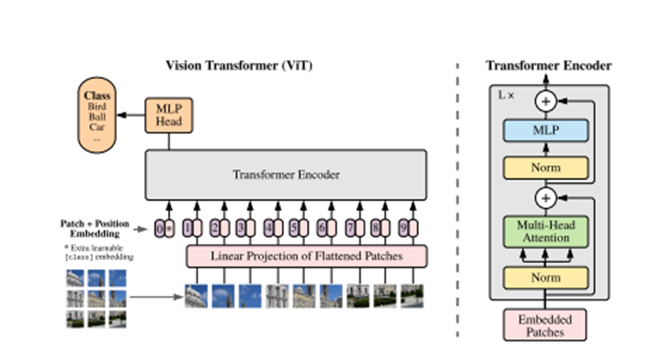
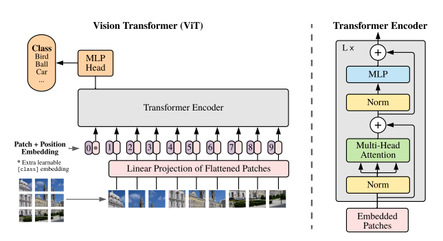
Figure 1: Model overview. We split an image into fixed-size patches, linearly embed each of them, add position embeddings, and feed the resulting sequence of vectors to a standard Transformer encoder. In order to perform classification, we use the standard approach of adding an extra learnable “classification token” to the sequence. The illustration of the Transformer encoder was inspired by Vaswani et al. (2017).
Figure 1: 모델 개요. 우리는 이미지를 고정 크기의 패치로 나누고, 각각을 선형으로 임베딩하고, 위치 임베딩을 추가한 후, 결과적인 벡터 시퀀스를 표준 Transformer 인코더에 입력합니다. 분류를 수행하기 위해, 시퀀스에 학습 가능한 "분류 토큰"을 추가하는 표준적인 접근 방식을 사용합니다. Transformer 인코더의 그림은 Vaswani et al. (2017)에 영감을 받아 작성되었습니다.
3. Method
In model design we follow the original Transformer (Vaswani et al., 2017) as closely as possible. An advantage of this intentionally simple setup is that scalable NLP Transformer architectures – and their efficient implementations – can be used almost out of the box.
모델 디자인에서는 가능한 한 원래의 Transformer (Vaswani et al., 2017)를 따르도록 노력했습니다. 이러한 의도적으로 간단한 설정의 장점은 확장 가능한 NLP Transformer 아키텍처와 효율적인 구현이 거의 그대로 사용될 수 있다는 점입니다.
3.1 VISION TRANSFORMER (VIT)
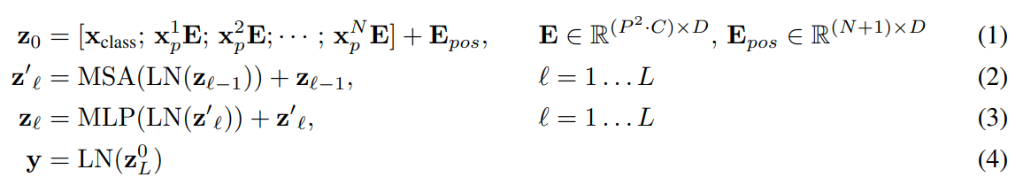
An overview of the model is depicted in Figure 1. The standard Transformer receives as input a 1D sequence of token embeddings. To handle 2D images, we reshape the image x ∈ R H×W×C into a sequence of flattened 2D patches xp ∈ R N×(P 2 ·C) , where (H, W) is the resolution of the original image, C is the number of channels, (P, P) is the resolution of each image patch, and N = HW/P2 is the resulting number of patches, which also serves as the effective input sequence length for the Transformer. The Transformer uses constant latent vector size D through all of its layers, so we flatten the patches and map to D dimensions with a trainable linear projection (Eq. 1). We refer to the output of this projection as the patch embeddings.
Similar to BERT’s [class] token, we prepend a learnable embedding to the sequence of embedded patches (z 0 0 = xclass), whose state at the output of the Transformer encoder (z 0 L ) serves as the image representation y (Eq. 4). Both during pre-training and fine-tuning, a classification head is attached to z 0 L . The classification head is implemented by a MLP with one hidden layer at pre-training time and by a single linear layer at fine-tuning time. Position embeddings are added to the patch embeddings to retain positional information. We use standard learnable 1D position embeddings, since we have not observed significant performance gains from using more advanced 2D-aware position embeddings (Appendix D.4). The resulting sequence of embedding vectors serves as input to the encoder.

Figure 1에서 모델의 개요를 보여줍니다. 표준 Transformer는 1D 토큰 임베딩 시퀀스를 입력으로 받습니다. 2D 이미지를 처리하기 위해 이미지 x ∈ R H×W×C를 평탄화된 2D 패치 시퀀스 xp ∈ R N×(P 2 ·C)로 재구성합니다. 여기서 (H, W)는 원래 이미지의 해상도, C는 채널의 수, (P, P)는 각 이미지 패치의 해상도를 나타내며, N = HW/P2는 패치의 개수로서 Transformer의 유효한 입력 시퀀스 길이로 사용됩니다. Transformer는 모든 레이어에서 일정한 잠재 벡터 크기 D를 사용하므로, 패치를 평탄화하고 학습 가능한 선형 변환(Eq. 1)을 사용하여 D 차원으로 매핑합니다. 이 변환의 출력을 패치 임베딩이라고 합니다.
Similar to BERT’s [class] token, we prepend a learnable embedding to the sequence of embedded patches (z 0 0 = xclass), whose state at the output of the Transformer encoder (z 0 L ) serves as the image representation y (Eq. 4). Both during pre-training and fine-tuning, a classification head is attached to z 0 L . The classification head is implemented by a MLP with one hidden layer at pre-training time and by a single linear layer at fine-tuning time. Position embeddings are added to the patch embeddings to retain positional information. We use standard learnable 1D position embeddings, since we have not observed significant performance gains from using more advanced 2D-aware position embeddings (Appendix D.4). The resulting sequence of embedding vectors serves as input to the encoder.
The Transformer encoder (Vaswani et al., 2017) consists of alternating layers of multiheaded selfattention (MSA, see Appendix A) and MLP blocks (Eq. 2, 3). Layernorm (LN) is applied before every block, and residual connections after every block (Wang et al., 2019; Baevski & Auli, 2019). The MLP contains two layers with a GELU non-linearity.
BERT와 유사하게, 임베딩된 패치 시퀀스에 학습 가능한 임베딩을 앞에 추가합니다 (z 0 0 = xclass). Transformer 인코더의 출력 상태 (z 0 L)는 이미지 표현 y로 사용됩니다 (Eq. 4). 사전 훈련 및 세부 조정 동안에는 분류 헤드가 z 0 L에 연결됩니다. 분류 헤드는 사전 훈련 시에는 하나의 은닉층을 가진 MLP로 구현되고, 세부 조정 시에는 단일 선형 층으로 구현됩니다.
위치 임베딩은 패치 임베딩에 추가되어 위치 정보를 보존합니다. 우리는 고급 2D-aware 위치 임베딩을 사용하는 것보다 표준 학습 가능한 1D 위치 임베딩을 사용합니다. (부록 D.4 참조) 덧붙여서, 임베딩 벡터의 결과 시퀀스는 인코더의 입력으로 사용됩니다.
→ 1D positional embedding: 왼쪽 위부터 오른쪽 아래와 같이 차례로 순서를 매기는 것을 의미
→ 2D positional embedding: 2차원에 대해 x,y축에 대한 좌표가 있는 positional embedding
→ relative positional embedding: 패치들 사이의 상대적 거리를 활용한 positional embedding
Transformer 인코더 (Vaswani et al., 2017)는 다중 헤드 셀프 어텐션(MSA, 부록 A 참조)과 MLP 블록(Eq. 2, 3)이 번갈아 나오는 여러 개의 층으로 구성됩니다. 각 층은 레이어 정규화(LN)가 앞에 적용되며, 잔차 연결이 각 블록 뒤에 적용됩니다. (Wang et al., 2019; Baevski & Auli, 2019).
MLP 블록은 두 개의 완전 연결층으로 구성되며, GELU 비선형성을 가지고 있습니다. GELU 활성화 함수는 딥러닝 모델에서 비선형성을 도입하여 데이터의 복잡한 관계를 포착하는 데 효과적으로 사용됩니다.

→ z0: patch에 대한 정보 + position embedding의 합
→ z’l: normalization을 진행하고, multi-head self- attention 수행한 후, 잔차 더해줌
→ zl: normalization 한 번 더 수행 후, MLP 적용 후, 잔차 더해줌
→ y: 마지막 예측값에 normalization 한 번 더 적용
Inductive bias. We note that Vision Transformer has much less image-specific inductive bias than CNNs. In CNNs, locality, two-dimensional neighborhood structure, and translation equivariance are baked into each layer throughout the whole model. In ViT, only MLP layers are local and translationally equivariant, while the self-attention layers are global. The two-dimensional neighborhood structure is used very sparingly: in the beginning of the model by cutting the image into patches and at fine-tuning time for adjusting the position embeddings for images of different resolution (as described below). Other than that, the position embeddings at initialization time carry no information about the 2D positions of the patches and all spatial relations between the patches have to be learned from scratch.
인식 편향
Vision Transformer는 CNN에 비해 이미지 특정 인식 편향이 훨씬 적습니다. CNN에서는 각 레이어마다 지역성(locality), 2차원 이웃 구조, 이동 불변성(translation equivariance)이 전체 모델에 내재되어 있습니다. 반면에 ViT에서는 MLP(Multi-Layer Perceptron) 레이어만 지역적이고 이동 불변성을 가지며, self-attention 레이어는 전역적입니다. 2차원 이웃 구조는
매우 제한적으로 사용됩니다. 이미지를 패치(patch)로 잘라내어 모델의 시작 부분에서 사용하고, fine-tuning 시에는 다른 해상도를 가진 이미지에 대해 위치 임베딩을 조정하는 데 사용됩니다 (아래에서 설명됨). 초기화 단계에서 위치 임베딩은 패치의 2D 위치에 대한 정보를 전달하지 않으며, 패치 간의 모든 공간 관계는 처음부터 학습되어야 합니다.
→ VIT에서의 MLP는 이미 input에서 패치 단위로 입력값을 받기에 정보가 존재함.
→ self attention 레이어는 입력 시퀀스의 모든 위치 간의 상호작용을 수행함.
※ Self-attention은 입력 시퀀스 내의 각 위치가 다른 위치와 얼마나 관련되어 있는지를 계산하여 중요도를 부여함. 이를 통해 시퀀스 내의 임의의 위치가 전체 시퀀스의 다른 위치와 상호작용할 수 있음. 따라서 self-attention은 입력 시퀀스의 길이나 위치에 대해 상관없이 모든 위치 간의 관계를 모델링할 수 있으며, 이를 통해 전역적인 정보를 저장할 수 있음.
※ 반면에 MLP 레이어는 입력 위치와 직접적으로 연결되어 있으며, 지역적인 특징을 모델링함. 이 레이어는 입력 위치에 대한 특징 변환을 수행하므로, 이동 불변성을 가지게 됨. MLP는 입력 위치에 대해 독립적으로 작동하며, 입력의 순서나 위치에 영향을 받지 않음.
※ 아래 두 가지 방식을 통해 inductive bias가 주입됐다라고 말할 수 있음
→ patch extraction: 패치 단위로 분할하여, 순서가 존재하는 형태로 입력에 넣음 → 이를 통해 기존 MLP와는 다르게, locality와 translation equivariance가 내재됨.
→ resolution adjustment: fine tuning 시에 진행됨. 이미지의 크기에 따라 패치 크기는 동일하지만, 생성되는 패치 개수가 달라지기에, positional embedding을 조정해야됨 → 이를 통해 inductive bias가 주입.
Hybrid Architecture. As an alternative to raw image patches, the input sequence can be formed from feature maps of a CNN (LeCun et al., 1989). In this hybrid model, the patch embedding projection E (Eq. 1) is applied to patches extracted from a CNN feature map. As a special case, the patches can have spatial size 1x1, which means that the input sequence is obtained by simply flattening the spatial dimensions of the feature map and projecting to the Transformer dimension. The classification input embedding and position embeddings are added as described above.
혼합 아키텍처
원시 이미지 패치 대신, 입력 시퀀스를 CNN (LeCun et al., 1989)의 피쳐 맵(feature map)으로부터 구성할 수도 있습니다. 이 혼합 모델에서는 패치 임베딩 투영 E (식 1)이 CNN 피쳐 맵에서 추출한 패치에 적용됩니다. 특별한 경우로, 패치의 공간 크기가 1x1인 경우 입력 시퀀스는 단순히 피쳐 맵의 공간 차원을 펼쳐서 Transformer 차원으로 투영하는 것으로 얻어집니다. 분류 입력 임베딩과 위치 임베딩은 위에서 설명한 대로 추가됩니다.
→ VIT는 raw image가 아닌 CNN으로 추출한 raw image의 feature map을 활용하는 hybrid architecture로도 사용할 수 있음
→ feature map의 경우, 이미 raw image의 공간적 정보를 포함하고 있기에 hybrid architecture는 패치 크기를 1x1로 설정해도 됨
→ 1x1 패치를 사용할 경우 피처맵의 공간 차원을 flatten하여 각 벡터에 linear projection 적용하면 됨
3.2 FINE-TUNING AND HIGHER RESOLUTION Typically, we pre-train ViT on large datasets, and fine-tune to (smaller) downstream tasks. For this, we remove the pre-trained prediction head and attach a zero-initialized D × K feedforward layer, where K is the number of downstream classes. It is often beneficial to fine-tune at higher resolution than pre-training (Touvron et al., 2019; Kolesnikov et al., 2020). When feeding images of higher resolution, we keep the patch size the same, which results in a larger effective sequence length. The Vision Transformer can handle arbitrary sequence lengths (up to memory constraints), however, the pre-trained position embeddings may no longer be meaningful. We therefore perform 2D interpolation of the pre-trained position embeddings, according to their location in the original image. Note that this resolution adjustment and patch extraction are the only points at which an inductive bias about the 2D structure of the images is manually injected into the Vision Transformer.
3.2 파인튜닝과 고해상도 일반적으로, 우리는 ViT를 대규모 데이터셋에서 사전 훈련한 후 (더 작은) 하위 작업에 대해 파인튜닝합니다. 이를 위해, 사전 훈련된 예측 헤드를 제거하고 영벡터로 초기화된 D × K 피드포워드 레이어를 추가합니다. 여기서 K는 하위 작업의 클래스 수입니다. 사전 훈련보다 더 높은 해상도에서 파인튜닝하는 것이 종종 유리합니다 (Touvron et al., 2019; Kolesnikov et al., 2020). 더 높은 해상도의 이미지를 입력할 때, 패치 크기는 동일하게 유지하며, 이로 인해 더 큰 유효한 시퀀스 길이가 생성됩니다. Vision Transformer는 임의의 시퀀스 길이를 처리할 수 있지만, 사전 훈련된 위치 임베딩은 더 이상 의미가 없을 수 있습니다. 따라서, 사전 훈련된 위치 임베딩을 원래 이미지에서의 위치에 따라 2D 보간(interpolation)을 수행합니다. 이 때, 해상도 조정과 패치 추출은 이미지의 2D 구조에 대한 귀납적 편향이 Vision Transformer에 수동으로 주입되는 유일한 지점임에 유의합니다.
→ transformer encoder는 그대로 사용하되, MLP head (MLP의 출력을 입력으로 받아 최종 예측값 만드는 역할)을 0으로 초기화. (초기화 방법으로 생각하면 될 듯)
※ pre-trained prediction head: 이미지 분류 작업에서는 예측 헤드가 클래스 수에 해당하는 출력 노드를 가지고, 각 클래스에 대한 확률을 예측함.
→ ViT를 fine tuning 할 때, pre-training과 동일한 패치 크기를 사용하기 때문에, 고해상도 이미지로 fine-tuning을 할 경우, sequence의 길이가 더 길어짐.
→ ViT는 가변적 패치들을 처리할 수 있지만, pre-trained position embedding은 의미가 사라지기 때문에, pretrained position embedding을 원본 이미지 위치에 따라 이중 선형보간법 사용
4. Experiments
We evaluate the representation learning capabilities of ResNet, Vision Transformer (ViT), and the hybrid. To understand the data requirements of each model, we pre-train on datasets of varying size and evaluate many benchmark tasks. When considering the computational cost of pre-training the model, ViT performs very favourably, attaining state of the art on most recognition benchmarks at a lower pre-training cost. Lastly, we perform a small experiment using self-supervision, and show that self-supervised ViT holds promise for the future.
우리는 ResNet, Vision Transformer (ViT), 그리고 하이브리드 모델의 표현 학습 능력을 평가합니다. 각 모델의 데이터 요구 사항을 이해하기 위해 다양한 크기의 데이터셋에서 사전 훈련을 수행하고 여러 벤치마크 작업을 평가합니다. 모델의 사전 훈련 비용을 고려할 때, ViT는 매우 우수한 성능을 보여주며, 낮은 사전 훈련 비용으로 대부분의 인식 벤치마크에서 최고 성능을 달성합니다. 마지막으로, 우리는 자기 지도 학습을 사용한 작은 실험을 수행하고, 자기 지도 학습 ViT가 미래에 대한 약속을 보여줍니다.
4.1 SETUP Datasets.
To explore model scalability, we use the ILSVRC-2012 ImageNet dataset with 1k classes and 1.3M images (we refer to it as ImageNet in what follows), its superset ImageNet-21k with 21k classes and 14M images (Deng et al., 2009), and JFT (Sun et al., 2017) with 18k classes and 303M high-resolution images. We de-duplicate the pre-training datasets w.r.t. the test sets of the downstream tasks following Kolesnikov et al. (2020). We transfer the models trained on these dataset to several benchmark tasks: ImageNet on the original validation labels and the cleaned-up ReaL labels (Beyer et al., 2020), CIFAR-10/100 (Krizhevsky, 2009), Oxford-IIIT Pets (Parkhi et al., 2012), and Oxford Flowers-102 (Nilsback & Zisserman, 2008). For these datasets, pre-processing follows Kolesnikov et al. (2020). We also evaluate on the 19-task VTAB classification suite (Zhai et al., 2019b). VTAB evaluates low-data transfer to diverse tasks, using 1 000 training examples per task. The tasks are divided into three groups: Natural – tasks like the above, Pets, CIFAR, etc. Specialized – medical and satellite imagery, and Structured – tasks that require geometric understanding like localization.
모델의 확장성을 탐구하기 위해, 우리는 다양한 데이터셋을 사용합니다. ILSVRC-2012 ImageNet 데이터셋은 1,000개 클래스와 1.3백만 장의 이미지로 구성되어 있습니다. ImageNet의 상위 집합인 ImageNet-21k는 21,000개 클래스와 14백만 장의 이미지로 이루어져 있습니다. 또한, JFT 데이터셋은 18,000개 클래스와 3억 3천만 개의 고해상도 이미지로 구성되어 있습니다.
실험의 공정성을 보장하기 위해, 우리는 사전 훈련 데이터셋과 후속 작업의 테스트 세트 사이에서 중복된 이미지를 제거합니다. 이는 Kolesnikov 등의 접근 방식을 따릅니다. 그리고 이러한 사전 훈련 모델을 여러 벤치마크 작업에 전이합니다. 벤치마크 작업에는 ImageNet (원래의 검증 레이블과 정제된 ReaL 레이블), CIFAR-10/100, Oxford-IIIT Pets, Oxford Flowers-102가 포함됩니다. 이러한 데이터셋에 대한 사전 처리 단계는 Kolesnikov 등의 방법론을 따릅니다.
또한, VTAB 분류 스위트에서도 모델을 평가합니다. VTAB는 19개의 작업으로 구성되어 있으며, 각 작업에는 1,000개의 훈련 예제만 사용됩니다. 이 작업들은 세 가지 그룹으로 나뉘어 있습니다. Natural 그룹에는 Pets, CIFAR 등과 같은 작업이 포함되어 있으며, Specialized 그룹에는 의료 및 위성 이미지 작업이 포함되어 있습니다. 그리고 Structured 그룹에는 지오메트리 이해와 로컬라이제이션이 필요한 작업이 포함되어 있습니다.
Model Variants. We base ViT configurations on those used for BERT (Devlin et al., 2019), as summarized in Table 1. The “Base” and “Large” models are directly adopted from BERT and we add the larger “Huge” model. In what follows we use brief notation to indicate the model size and the input patch size: for instance, ViT-L/16 means the “Large” variant with 16×16 input patch size. Note that the Transformer’s sequence length is inversely proportional to the square of the patch size, thus models with smaller patch size are computationally more expensive. For the baseline CNNs, we use ResNet (He et al., 2016), but replace the Batch Normalization layers (Ioffe & Szegedy, 2015) with Group Normalization (Wu & He, 2018), and used standardized convolutions (Qiao et al., 2019). These modifications improve transfer (Kolesnikov et al., 2020), and we denote the modified model “ResNet (BiT)”. For the hybrids, we feed the intermediate feature maps into ViT with patch size of one “pixel”. To experiment with different sequence lengths, we either (i) take the output of stage 4 of a regular ResNet50 or (ii) remove stage 4, place the same number of layers in stage 3 (keeping the total number of layers), and take the output of this extended stage 3. Option (ii) results in a 4x longer sequence length, and a more expensive ViT model.
ViT 구성은 BERT에 사용된 구성을 기반으로 하며, 이는 Table 1에 요약되어 있습니다. "Base"와 "Large" 모델은 BERT에서 직접 채용되었으며, 우리는 더 큰 "Huge" 모델을 추가합니다. 이후에는 모델 크기와 입력 패치 크기를 간단하게 표기하여 사용합니다. 예를 들어, ViT-L/16은 16x16 입력 패치 크기를 가진 "Large" 변형 모델을 의미합니다. 패치 크기의 제곱에 반비례하는 트랜스포머의 시퀀스 길이를 유의해야 합니다. 따라서 패치 크기가 작은 모델일수록 계산 비용이 더 많이 듭니다.
기준이 되는 CNN으로는 ResNet (He 등, 2016)을 사용하지만, Batch Normalization 레이어(Ioffe & Szegedy, 2015)를 Group Normalization (Wu & He, 2018)으로 대체하고, 표준화된 합성곱(Qiao 등, 2019)을 사용합니다. 이러한 수정 사항은 전이 학습을 개선하며, 수정된 모델을 "ResNet (BiT)"라고 표기합니다. 하이브리드 모델의 경우 중간 특성 맵을 한 개의 "픽셀" 크기의 패치로 ViT에 전달합니다. 다른 시퀀스 길이를 실험하기 위해, (i) 일반적인 ResNet50의 stage 4의 출력을 사용하거나 (ii) stage 4를 제거하고 동일한 수의 레이어를 stage 3에 배치하고 이 확장된 stage 3의 출력을 사용합니다. (ii) 옵션은 4배 더 긴 시퀀스 길이와 더 비싼 ViT 모델을 만들어냅니다.
Training & Fine-tuning. We train all models, including ResNets, using Adam (Kingma & Ba, 2015) with β1 = 0.9, β2 = 0.999, a batch size of 4096 and apply a high weight decay of 0.1, which we found to be useful for transfer of all models (Appendix D.1 shows that, in contrast to common practices, Adam works slightly better than SGD for ResNets in our setting). We use a linear learning rate warmup and decay, see Appendix B.1 for details. For fine-tuning we use SGD with momentum, batch size 512, for all models, see Appendix B.1.1. For ImageNet results in Table 2, we fine-tuned at higher resolution: 512 for ViT-L/16 and 518 for ViT-H/14, and also used Polyak & Juditsky (1992) averaging with a factor of 0.9999 (Ramachandran et al., 2019; Wang et al., 2020b).
훈련 및 파인튜닝. 우리는 ResNet을 포함한 모든 모델을 Adam (Kingma & Ba, 2015)을 사용하여 훈련합니다. 이때 β1 = 0.9, β2 = 0.999, 배치 크기는 4096이며, 가중치 감쇠(weight decay)로는 0.1을 적용합니다. 이는 모든 모델의 전이 학습에 유용하다는 것을 발견하였습니다 (부록 D.1에서는 일반적인 관행과는 다르게, Adam이 우리의 설정에서 ResNet에 대해 SGD보다 약간 더 잘 작동한다는 것을 보여줍니다). 선형 학습률 웜업과 감소를 사용하며, 자세한 내용은 부록 B.1을 참조하십시오. 파인튜닝에는 SGD와 모멘텀을 사용하며, 모든 모델에 대해 배치 크기는 512로 설정합니다. 자세한 내용은 부록 B.1.1을 참조하십시오. Table 2의 ImageNet 결과에서는 더 높은 해상도에서 파인튜닝을 진행하였습니다. ViT-L/16의 경우 512, ViT-H/14의 경우 518로 설정하였으며, Polyak & Juditsky (1992) 평균화를 0.9999의 비율로 사용하였습니다 (Ramachandran et al., 2019; Wang et al., 2020b).
Metrics. We report results on downstream datasets either through few-shot or fine-tuning accuracy. Fine-tuning accuracies capture the performance of each model after fine-tuning it on the respective dataset. Few-shot accuracies are obtained by solving a regularized least-squares regression problem that maps the (frozen) representation of a subset of training images to {−1, 1} K target vectors. This formulation allows us to recover the exact solution in closed form. Though we mainly focus on fine-tuning performance, we sometimes use linear few-shot accuracies for fast on-the-fly evaluation where fine-tuning would be too costly.
우리는 다운스트림 데이터셋에 대한 결과를 표시할 때 적은 데이터셋(few-shot) 또는 파인튜닝 정확도를 사용합니다. 파인튜닝 정확도는 각 모델을 해당 데이터셋에 파인튜닝한 후의 성능을 측정합니다. 적은 데이터셋 정확도는 (고정된) 일부 훈련 이미지의 표현을 {−1, 1} K의 목표 벡터에 매핑하는 정규화된 최소제곱 회귀 문제를 해결하여 얻습니다. 이러한 수식은 닫힌 형태로 정확한 솔루션을 복구할 수 있게 합니다. 우리는 주로 파인튜닝 성능에 초점을 두지만, 파인튜닝이 너무 비용이 많이 드는 경우에는 선형적인 적은 데이터셋 정확도를 사용하여 빠르게 실시간으로 평가합니다.
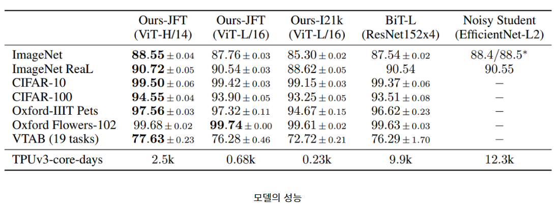
4.2 COMPARISON TO STATE OF THE ART We first compare our largest models – ViT-H/14 and ViT-L/16 – to state-of-the-art CNNs from the literature. The first comparison point is Big Transfer (BiT) (Kolesnikov et al., 2020), which performs supervised transfer learning with large ResNets. The second is Noisy Student (Xie et al., 2020), which is a large EfficientNet trained using semi-supervised learning on ImageNet and JFT300M with the labels removed. Currently, Noisy Student is the state of the art on ImageNet and BiT-L on the other datasets reported here. All models were trained on TPUv3 hardware, and we report the number of TPUv3-core-days taken to pre-train each of them, that is, the number of TPU v3 cores (2 per chip) used for training multiplied by the training time in days. Table 2 shows the results. The smaller ViT-L/16 model pre-trained on JFT-300M outperforms BiT-L (which is pre-trained on the same dataset) on all tasks, while requiring substantially less computational resources to train. The larger model, ViT-H/14, further improves the performance, especially on the more challenging datasets – ImageNet, CIFAR-100, and the VTAB suite. Interestingly, this model still took substantially less compute to pre-train than prior state of the art. However, we note that pre-training efficiency may be affected not only by the architecture choice, but also other parameters, such as training schedule, optimizer, weight decay, etc. We provide a controlled study of performance vs. compute for different architectures in Section 4.4. Finally, the ViT-L/16 model pre-trained on the public ImageNet-21k dataset performs well on most datasets too, while taking fewer resources to pre-train: it could be trained using a standard cloud TPUv3 with 8 cores in approximately 30 days.
4.2 최신 기술과의 비교 우선 가장 큰 모델인 ViT-H/14와 ViT-L/16을 문헌에서 제시된 최신 CNN과 비교합니다. 첫 번째 비교 대상은 Big Transfer (BiT) (Kolesnikov et al., 2020)입니다. BiT는 큰 ResNet을 사용한 지도 전이 학습을 수행합니다. 두 번째는 Noisy Student (Xie et al., 2020)로, 이는 ImageNet 및 JFT300M에서 라벨을 제거한 상태로 준지도 학습을 수행하는 큰 EfficientNet입니다. 현재, Noisy Student는 ImageNet에서 최신 기술이며, 다른 데이터셋에서는 BiT-L이 최신 기술입니다. 모든 모델은 TPUv3 하드웨어에서 훈련되었으며, 각각의 사전 훈련에 소요된 TPUv3 코어-일 수를 보고합니다. 이는 훈련에 사용된 TPU v3 코어(칩당 2개)의 개수를 훈련 기간(일)으로 곱한 값입니다. Table 2는 이러한 결과를 보여줍니다. JFT-300M에서 사전 훈련된 작은 ViT-L/16 모델은 모든 작업에서 동일한 데이터셋에서 사전 훈련된 BiT-L보다 우수한 성능을 발휘하며, 훈련에 필요한 계산 자원은 훨씬 적습니다. 더 큰 모델인 ViT-H/14은 특히 ImageNet, CIFAR-100 및 VTAB 스위트와 같은 더 도전적인 데이터셋에서 성능을 더욱 향상시킵니다. 흥미롭게도, 이 모델은 여전히 사전 훈련에 이전의 최신 기술보다 훨씬 적은 계산 리소스를 사용했습니다. 그러나 사전 훈련 효율성은 아키텍처 선택뿐만 아니라 훈련 일정, 옵티마이저, 가중치 감쇠 등 다른 매개변수에도 영향을 받을 수 있음을 참고해야 합니다. 서로 다른 아키텍처에 대한 성능 대 계산 비교에 대한 제어된 연구를 4.4절에서 제공합니다. 마지막으로, 공개된 ImageNet-21k 데이터셋에서 사전 훈련된 ViT-L/16 모델은 대부분의 데이터셋에서도 잘 수행되며, 사전 훈련에 필요한 자원은 적습니다. 일반적인 클라우드 TPUv3 (8개 코어)를 사용하여 약 30일 동안 훈련할 수 있었습니다.
Figure 2 decomposes the VTAB tasks into their respective groups, and compares to previous SOTA methods on this benchmark: BiT, VIVI – a ResNet co-trained on ImageNet and Youtube (Tschannen et al., 2020), and S4L – supervised plus semi-supervised learning on ImageNet (Zhai et al., 2019a). ViT-H/14 outperforms BiT-R152x4, and other methods, on the Natural and Structured tasks. On the Specialized the performance of the top two models is similar.
Figure 2 분해 VTAB 작업을 해당 그룹으로 나누고 이 벤치마크에 대한 이전 SOTA 방법과 비교합니다: BiT, VIVI - ImageNet과 Youtube에서 공동으로 훈련된 ResNet (Tschannen et al., 2020) 및 S4L - ImageNet에서 지도 및 준지도 학습 (Zhai et al., 2019a). ViT-H/14는 BiT-R152x4 및 다른 방법들에 비해 Natural 및 Structured 작업에서 우수한 성능을 보입니다. Specialized 작업에서 상위 두 모델의 성능은 유사합니다.
4.3 PRE-TRAINING DATA REQUIREMENTS The Vision Transformer performs well when pre-trained on a large JFT-300M dataset. With fewer inductive biases for vision than ResNets, how crucial is the dataset size? We perform two series of experiments. First, we pre-train ViT models on datasets of increasing size: ImageNet, ImageNet-21k, and JFT300M. To boost the performance on the smaller datasets, we optimize three basic regularization parameters – weight decay, dropout, and label smoothing. Figure 3 shows the results after finetuning to ImageNet (results on other datasets are shown in Table 5)2 . When pre-trained on the smallest dataset, ImageNet, ViT-Large models underperform compared to ViT-Base models, despite (moderate) regularization. With ImageNet-21k pre-training, their performances are similar. Only with JFT-300M, do we see the full benefit of larger models. Figure 3 also shows the performance region spanned by BiT models of different sizes. The BiT CNNs outperform ViT on ImageNet, but with the larger datasets, ViT overtakes. Second, we train our models on random subsets of 9M, 30M, and 90M as well as the full JFT300M dataset. We do not perform additional regularization on the smaller subsets and use the same hyper-parameters for all settings. This way, we assess the intrinsic model properties, and not the effect of regularization. We do, however, use early-stopping, and report the best validation accuracy achieved during training. To save compute, we report few-shot linear accuracy instead of full finetuning accuracy. Figure 4 contains the results. Vision Transformers overfit more than ResNets with comparable computational cost on smaller datasets. For example, ViT-B/32 is slightly faster than ResNet50; it performs much worse on the 9M subset, but better on 90M+ subsets. The same is true for ResNet152x2 and ViT-L/16. This result reinforces the intuition that the convolutional inductive bias is useful for smaller datasets, but for larger ones, learning the relevant patterns directly from data is sufficient, even beneficial. Overall, the few-shot results on ImageNet (Figure 4), as well as the low-data results on VTAB (Table 2) seem promising for very low-data transfer. Further analysis of few-shot properties of ViT is an exciting direction of future work.
비전 트랜스포머(Vision Transformer)는 대용량 JFT-300M 데이터셋으로 사전 학습 시 우수한 성능을 보입니다. ResNet과 비교하여 비전에 대한 귀납적 편향이 적은 트랜스포머 모델에서 데이터셋의 크기는 얼마나 중요한지 알아보기 위해 두 가지 실험을 수행합니다.
첫 번째로, ViT 모델을 ImageNet, ImageNet-21k 및 JFT300M과 같은 크기의 데이터셋에서 사전 학습합니다. 작은 데이터셋에서의 성능을 향상시키기 위해 가중치 감소(weight decay), 드롭아웃(dropout), 라벨 스무딩(label smoothing)과 같은 세 가지 기본적인 정규화 매개변수를 최적화합니다. Figure 3은 ImageNet으로의 파인튜닝 이후의 결과를 보여줍니다(다른 데이터셋의 결과는 테이블 5에 표시됩니다). 가장 작은 데이터셋인 ImageNet으로 사전 학습할 때, ViT-Large 모델은 (적당한 정규화에도 불구하고) ViT-Base 모델보다 성능이 떨어집니다. ImageNet-21k 사전 학습 시 두 모델의 성능이 유사해집니다. 그러나 JFT-300M 사전 학습 시에만 큰 모델의 모든 이점을 확인할 수 있습니다. Figure 3은 다양한 크기의 BiT 모델에 대한 성능 범위도 보여줍니다. BiT CNN은 ImageNet에서 ViT보다 우수한 성능을 보입니다. 그러나 데이터셋의 크기가 커질수록 ViT가 BiT 모델을 앞지를 수 있습니다.
두 번째로, 9M, 30M, 90M 및 JFT300M의 무작위 하위 데이터셋에서 모델을 훈련합니다. 작은 하위 데이터셋에 대해서는 추가적인 정규화를 수행하지 않으며, 모든 설정에 동일한 하이퍼파라미터를 사용합니다. 이렇게 함으로써 모델의 본질적인 특성을 평가하고, 정규화의 영향이 아닌 모델의 특성을 알아볼 수 있습니다. 훈련 중에 최상의 검증 정확도를 기록하기 위해 조기 종료를 사용하며, 계산량을 줄이기 위해 완전한 파인튜닝 정확도 대신 few-shot 선형 정확도를 보고합니다. Figure 4는 이러한 결과를 담고 있습니다. 비전 트랜스포머는 비슷한 계산 비용을 갖는 ResNet과 비교하여 작은 데이터셋에서 과적합 현상이 더 많이 발생합니다. 예를 들어, ViT-B/32는 ResNet50보다 약간 더 빠르지만 9M 하위 데이터셋에서 성능이 크게 저하되고 90M 이상의 하위 데이터셋에서는 더 좋은 성능을 보입니다. ResNet152x2와 ViT-L/16에 대해서도 동일한 경향이 나타납니다. 이 결과는 합성곱적 편향이 작은 데이터셋에 유용하지만, 큰 데이터셋에 대해서는 데이터로부터 직접 관련 패턴을 학습하는 것이 충분하며 심지어 이점이 있다는 직관을 강화시킵니다.
Overall, the few-shot results on ImageNet (Figure 4), as well as the low-data results on VTAB (Table 2) seem promising for very low-data transfer. Further analysis of few-shot properties of ViT is an exciting direction of future work.
전반적으로, ImageNet에서의 소수샷 결과 (Figure 4) 및 VTAB에서의 저량 데이터 결과 (Table 2)는 매우 적은 데이터 전이에 대한 유망한 가능성을 보여줍니다. ViT의 소수샷 특성에 대한 추가적인 분석은 향후 연구의 흥미로운 방향입니다.
4.4 SCALING STUDY We perform a controlled scaling study of different models by evaluating transfer performance from JFT-300M. In this setting data size does not bottleneck the models’ performances, and we assess performance versus pre-training cost of each model. The model set includes: 7 ResNets, R50x1, R50x2 R101x1, R152x1, R152x2, pre-trained for 7 epochs, plus R152x2 and R200x3 pre-trained for 14 epochs; 6 Vision Transformers, ViT-B/32, B/16, L/32, L/16, pre-trained for 7 epochs, plus L/16 and H/14 pre-trained for 14 epochs; and 5 hybrids, R50+ViT-B/32, B/16, L/32, L/16 pretrained for 7 epochs, plus R50+ViT-L/16 pre-trained for 14 epochs (for hybrids, the number at the end of the model name stands not for the patch size, but for the total dowsampling ratio in the ResNet backbone). Figure 5 contains the transfer performance versus total pre-training compute (see Appendix D.5 for details on computational costs). Detailed results per model are provided in Table 6 in the Appendix. A few patterns can be observed. First, Vision Transformers dominate ResNets on the performance/compute trade-off. ViT uses approximately 2 − 4× less compute to attain the same performance (average over 5 datasets). Second, hybrids slightly outperform ViT at small computational budgets, but the difference vanishes for larger models. This result is somewhat surprising, since one might expect convolutional local feature processing to assist ViT at any size. Third, Vision Transformers appear not to saturate within the range tried, motivating future scaling efforts.
4.4 스케일링 연구 우리는 JFT-300M으로부터의 전이 성능을 평가하여 다양한 모델의 제어된 스케일링 연구를 수행합니다. 이 설정에서는 데이터 크기가 모델의 성능에 영향을 미치지 않으며, 각 모델의 사전 훈련 비용 대비 성능을 평가합니다. 모델 세트에는 다음이 포함됩니다. 7개의 ResNet 모델인 R50x1, R50x2, R101x1, R152x1, R152x2, 각각 7개의 epoch에 대해 사전 훈련된 모델과 R152x2와 R200x3는 14개의 epoch에 대해 사전 훈련된 모델; 6개의 Vision Transformer 모델인 ViT-B/32, B/16, L/32, L/16, 각각 7개의 epoch에 대해 사전 훈련된 모델과 L/16 및 H/14는 14개의 epoch에 대해 사전 훈련된 모델; 그리고 5개의 하이브리드 모델인 R50+ViT-B/32, B/16, L/32, L/16은 각각 7개의 epoch에 대해 사전 훈련된 모델과 R50+ViT-L/16은 14개의 epoch에 대해 사전 훈련된 모델입니다 (하이브리드 모델의 경우 모델 이름 끝의 숫자는 패치 크기가 아닌 ResNet 백본의 전체 다운샘플링 비율을 나타냅니다).
Figure 5에는 전이 성능 대비 총 사전 훈련 컴퓨트(컴퓨팅 비용에 대한 자세한 내용은 부록 D.5를 참조)가 포함되어 있습니다. 모델별 자세한 결과는 부록의 Table 6에서 제공됩니다. 몇 가지 패턴을 관찰할 수 있습니다. 첫째, 비전 트랜스포머는 성능/컴퓨트 교환에서 ResNet을 압도합니다. ViT는 동일한 성능을 달성하기 위해 약 2~4배 더 적은 컴퓨트를 사용합니다(5개 데이터셋에 대한 평균). 둘째, 하이브리드 모델은 작은 컴퓨팅 예산에서 ViT보다 약간 우수한 성능을 보이지만, 더 큰 모델에 대해서는 차이가 사라집니다. 이 결과는 한편으로는 컨볼루션 지역 특징 처리가 어떤 크기에서든 ViT를 지원할 것으로 예상할 수 있기 때문에 다소 놀라운 것입니다. 셋째, Vision Transformer는 시도한 범위 내에서 포화되지 않는 것으로 나타나며, 향후 스케일링 연구를 독려합니다.
4.5 INSPECTING VISION TRANSFORMER To begin to understand how the Vision Transformer processes image data, we analyze its internal representations. The first layer of the Vision Transformer linearly projects the flattened patches into a lower-dimensional space (Eq. 1). Figure 7 (left) shows the top principal components of the the learned embedding filters. The components resemble plausible basis functions for a low-dimensional representation of the fine structure within each patch. After the projection, a learned position embedding is added to the patch representations. Figure 7 (center) shows that the model learns to encode distance within the image in the similarity of position embeddings, i.e. closer patches tend to have more similar position embeddings. Further, the row-column structure appears; patches in the same row/column have similar embeddings. Finally, a sinusoidal structure is sometimes apparent for larger grids (Appendix D). That the position embeddings learn to represent 2D image topology explains why hand-crafted 2D-aware embedding variants do not yield improvements (Appendix D.4). Self-attention allows ViT to integrate information across the entire image even in the lowest layers. We investigate to what degree the network makes use of this capability. Specifically, we compute the average distance in image space across which information is integrated, based on the attention weights (Figure 7, right). This “attention distance” is analogous to receptive field size in CNNs. We find that some heads attend to most of the image already in the lowest layers, showing that the ability to integrate information globally is indeed used by the model. Other attention heads have consistently small attention distances in the low layers. This highly localized attention is less pronounced in hybrid models that apply a ResNet before the Transformer (Figure 7, right), suggesting that it may serve a similar function as early convolutional layers in CNNs. Further, the attention distance increases with network depth. Globally, we find that the model attends to image regions that are semantically relevant for classification (Figure 6).
4.5 비전 트랜스포머의 내부 표현 분석 비전 트랜스포머가 이미지 데이터를 처리하는 방식을 이해하기 위해 내부 표현을 분석합니다. 비전 트랜스포머의 첫 번째 레이어는 패치들을 낮은 차원의 공간으로 선형 투영합니다 (식 1). Figure 7 (왼쪽)은 학습된 임베딩 필터의 상위 주성분을 보여줍니다. 이 주성분들은 각 패치 내의 세부 구조의 저차원 표현을 위한 타당한 기저 함수와 유사합니다. 투영 이후, 학습된 위치 임베딩이 패치 표현에 추가됩니다. Figure 7 (가운데)은 모델이 위치 임베딩의 유사성을 통해 이미지 내의 거리를 인코딩하는 것을 보여줍니다. 즉, 더 가까운 패치는 보다 유사한 위치 임베딩을 갖습니다. 또한 행-열 구조가 나타납니다. 같은 행/열에 있는 패치들은 유사한 임베딩을 갖습니다. 마지막으로, 더 큰 그리드에 대해서는 때로 사인 함수 구조가 확인됩니다 (부록 D 참조). 위치 임베딩이 2D 이미지 토폴로지를 표현하는 방식을 학습한다는 것은 수동으로 만든 2D-aware 임베딩 변형이 개선되지 않는 이유를 설명합니다 (부록 D.4). 셀프 어텐션은 ViT가 최하위 레이어에서도 전체 이미지를 통합하는 능력을 제공합니다. 우리는 네트워크가 이 능력을 어느 정도 활용하는지 조사합니다. 특히, 어텐션 가중치를 기반으로 이미지 공간에서 정보가 통합되는 평균 거리를 계산합니다 (Figure 7, 오른쪽). 이 "어텐션 거리"는 CNN에서의 수용장 크기에 해당합니다. 일부 헤드는 이미 최하위 레이어에서 이미지의 대부분에 어텐션을 주는 것으로 나타납니다. 이는 모델이 실제로 정보를 전역적으로 통합하는 능력을 사용한다는 것을 보여줍니다. 다른 어텐션 헤드는 최하위 레이어에서 일관되게 작은 어텐션 거리를 가지고 있습니다. 이러한 고도로 국부화된 어텐션은 트랜스포머 이전에 ResNet을 적용하는 하이브리드 모델에서는 그 정도가 덜한 것으로 나타납니다 (Figure 7, 오른쪽), 이는 이러한 어텐션 거리가 CNN의 초기 합성곱 레이어와 유사한 기능을 수행할 수도 있다는 것을 시사합니다. 더 나아가, 어텐션 거리는 네트워크의 깊이와 함께 증가합니다. 전체적으로 모델은 분류에 의미 있는 시맨틱한 이미지 영역에 어텐션을 집중합니다 (Figure 6).
4.6 SELF-SUPERVISION
Transformers show impressive performance on NLP tasks. However, much of their success stems not only from their excellent scalability but also from large scale self-supervised pre-training (Devlinet al., 2019; Radford et al., 2018). We also perform a preliminary exploration on masked patch prediction for self-supervision, mimicking the masked language modeling task used in BERT. With self-supervised pre-training, our smaller ViT-B/16 model achieves 79.9% accuracy on ImageNet, a significant improvement of 2% to training from scratch, but still 4% behind supervised pre-training. Appendix B.1.2 contains further details. We leave exploration of contrastive pre-training (Chen et al., 2020b; He et al., 2020; Bachman et al., 2019; Henaff et al., 2020) to future work.
4.6 자기-감독 학습 트랜스포머는 NLP 작업에서 인상적인 성능을 보입니다. 그러나 그들의 성공은 우수한 확장성 뿐만 아니라 대규모 자기-감독 사전 학습 (Devlin et al., 2019; Radford et al., 2018) 에서도 기인합니다. 우리는 자기-감독 학습을 위해 마스크된 패치 예측에 대한 예비적인 탐색을 수행합니다. 이는 BERT에서 사용되는 마스크된 언어 모델링 작업을 모방한 것입니다. 자기-감독 사전 학습을 통해 작은 ViT-B/16 모델은 ImageNet에서 79.9%의 정확도를 달성하며, 처음부터 학습하는 것보다 2%의 상당한 개선을 보입니다. 그러나 여전히 지도 학습 사전 학습보다 4% 뒤쳐집니다. 부록 B.1.2에는 더 자세한 내용이 포함되어 있습니다. 대조적 사전 학습 (Chen et al., 2020b; He et al., 2020; Bachman et al., 2019; Henaff et al., 2020)의 탐구는 향후 연구로 남겨둡니다.
5. Conclusion
We have explored the direct application of Transformers to image recognition. Unlike prior works using self-attention in computer vision, we do not introduce image-specific inductive biases into the architecture apart from the initial patch extraction step. Instead, we interpret an image as a sequence of patches and process it by a standard Transformer encoder as used in NLP. This simple, yet scalable, strategy works surprisingly well when coupled with pre-training on large datasets. Thus, Vision Transformer matches or exceeds the state of the art on many image classification datasets, whilst being relatively cheap to pre-train.
While these initial results are encouraging, many challenges remain. One is to apply ViT to other computer vision tasks, such as detection and segmentation. Our results, coupled with those in Carion et al. (2020), indicate the promise of this approach. Another challenge is to continue exploring selfsupervised pre-training methods. Our initial experiments show improvement from self-supervised pre-training, but there is still large gap between self-supervised and large-scale supervised pretraining. Finally, further scaling of ViT would likely lead to improved performance.
저희는 Transformer를 직접적으로 이미지 인식에 적용해 보았습니다. 이전 연구들과는 달리, 이미지 특정의 귀납적 편향을 초기 패치 추출 단계를 제외하고 아키텍처에 도입하지 않았습니다. 대신, 이미지를 패치의 시퀀스로 해석하고 NLP에서 사용되는 표준 Transformer 인코더로 처리했습니다. 이러한 간단하면서도 확장 가능한 전략은 대용량 데이터셋에서의 사전 학습과 결합할 때 놀랍도록 잘 작동합니다. 따라서 Vision Transformer는 많은 이미지 분류 데이터셋에서 최신 기술 수준을 달성하거나 뛰어넘으며, 상대적으로 사전 학습 비용이 저렴합니다.
이 초기 결과는 격려되는 결과이지만, 많은 도전 과제들이 남아 있습니다. 하나는 ViT를 탐지 및 세그멘테이션과 같은 다른 컴퓨터 비전 작업에 적용하는 것입니다. 우리의 결과와 Carion et al. (2020)의 결과는 이 접근 방식의 잠재력을 보여줍니다. 또 다른 도전은 자기-감독 사전 학습 방법을 계속 탐구하는 것입니다. 초기 실험 결과는 자기-감독 사전 학습에서의 개선을 보여주지만, 자기-감독 사전 학습과 대규모 지도 학습 사전 학습 사이에는 여전히 큰 격차가 남아 있습니다. 마지막으로, ViT의 추가적인 확장은 성능 향상으로 이어질 것으로 예상됩니다.
1. Intro
- Transformer 구조의 NLP task에서의 성공
- 하지만, Computer Vision Task에서는 제대로 적용이 이루어지지 않음.
- Self-Attention을 추가한 CNN 계열 모델 구조와 아예 convolution을 attention으로 대체한 구조들이 제안됨. 그러나, 이론적으로는 효율성이 보장되었지만 실제 하드웨어 가속기와의 호환성이 떨어짐.
⇒ 이미지를 패치(patch)로 분할하고, 이러한 패치들의 선형 임베딩(sequence of linear embeddings)을 Transformer의 입력으로 제공. 이미지 패치는 NLP 응용프로그램에서의 토큰(단어)과 동일하게 처리시키고자 함.
📌 Inductive bias
: 학습 시 만나보지 못했던 상황에 대해 정확한 예측을 하기 위해 사용하는 추가적인 가정을 의미함 (사전 정보를 통해 추가된 가정)
- CNN: Vision 정보는 인접 픽셀간의 locality(근접 픽셀끼리의 종속성)가 존재한다는 것을 미리 알고 있기 때문에 Conv는 인접 픽셀간의 정보를 추출하기 위한 목적으로 설계되어 Conv의 inductive bias가 local 영역에서 spatial 정보를 잘 뽑아냄.+ transitional Invariance(사물 위치가 바뀌어도 동일 사물 인식)등의 특성을 가지기 때문에 이미지 데이터에 적합한 모델임
- 반면, MLP의 경우, all(input)-to-all (output) 관계로 모든 weight가 독립적이며 공유되지 않아 inductive bias가 매우 약함.
- Transformer는 attention을 통해 입력 데이터의 모든 요소간의 관계를 계산하므로 CNN보다는 Inductive Bias가 작다라고 할 수 있음.
→ CNN > Transformer > Fully Connected
→ inductive bias가 커질수록 generalizaion이 떨어짐 (둘은 trade off 관계)

2. Related Work
1. NLP
- Vaswani et al. (2017): Transformer 구조를 기계 번역 모델로 처음 제안. 현재 많은 NLP Task에서 가장 좋은 성능을 보여주는 구조
- Devlin et al. (2019): BERT를 제안. 노이즈를 제거하는 자기지도 사전학습을 수행.
- GPT 계열 (2018, 2019, 2020): 언어 모델을 사전학습 태스크로 선정하여 수행.
2. Computer Vision
- self-attention을 이미지에 단순 적용하는 방식은 해당 픽셀과 모든 픽셀 간의 attention weight을 구해야 하기 때문에 계산비용이 pixel 개수 n에 대하여 O(n2)의 복잡도를 가짐.
- Parmar et al. (2018): local neighborhood에만 self-attention을 적용.
- Sparse Transformers (2019), Weissenborn et al. (2019): attention의 범위를 scaling하는 방식으로 self-attention을 적용하고자 함.
→ 이러한 특별한 방식의 attention의 경우에는 하드웨어 가속기에서 연산을 효율적으로 수행하기에는 다소 번거로운 작업이 포함되어 있는 경우가 다수.
- Cordonnier et al. (2020): 이미지를 2x2의 패치로 쪼갠 후, 이에 self-attention을 적용함. 위와 같은 점에서 ViT와 매우 유사하나, 이미지 패치가 매우 작으므로 저해상도 입력 이미지에만 적용이 가능하다는 단점이 있음. ViT의 경우에는 중해상도 이미지를 다룰 수 있다는 점, Vanilla Transformer 구조를 차용해 기존의 SOTA CNN보다 더 좋은 성능을 증명해냈다는 점에서 해당 연구보다 우위를 가짐.
- image GPT (Chen et al., 2020): 이미지 해상도와 color space를 줄인 후, image pixel 단위로 Transformer를 적용한 생성 모델.
⇒ 기존 연구 대비 ViT의 차별점
- 표준 ImageNet 데이터셋보다 더 큰 크기의 데이터셋에서 image recognition 실험을 진행.
- 더 큰 크기의 데이터셋에서 학습시킴으로써 기존의 ResNet 기반 CNN보다 더 좋은 성능을 낼 수 있었음.
3. Method
- 모델에서는 원래의 transformer을 따르도록 노력하고자 했음.→ 이에 대한 장점: NLP transformer 아키텍처와 효율적인 구현이 거의 그대로 사용될 수 있음.
3.1) VISION TRANSFORMER (VIT)

- Transformer의 input 값은 1차원 시퀀스.
- 따라서 고정된 크기의 patch로 나눠준 이미지를 1차원 시퀀스로 flatten 해줘야 함
⇒ H*W*C → N*(P*P*C)로 변환ex) 256*256*3 ⇒ ((256*256)/9^2)* (9*9*3)
- ※ N(시퀀스 수) = H*W/(P^2) , P= 패치 개수
2) Step 2.
- 1차원 이미지를 Transformer에 사용할 수 있는 D차원의 벡터로 바꿔줌.→ 이 변환의 출력을 패치 임베딩이라고 함
3) Step 3.
- ( Learnable class embedding + 패치 embedding ) + position embedding
- learnable class embedding⇒ 임베딩된 패치 시퀀스에
학습가능한 임베딩을 앞에 추가시킴→ 모델의 파라미터로써 데이터의 특성과 작업에 맞게 최적화되는 값. 학습 과정에서 업데이트되는 가중치를 의미 → (이는 추후 이미지 전체에 대한 표현을 나타내게 됨)
- ※ 학습 가능한 임베딩을 사용하면 모델이 이미지 데이터의 패턴과 특징을 직접 학습하여 데이터에 맞는 효과적인 임베딩을 생성할 수 있음.
- position embedding→ 1D positional embedding: 왼쪽 위부터 오른쪽 아래와 같이 차례로 순서를 매기는 것을 의미 → relative positional embedding: 패치들 사이의 상대적 거리를 활용한 positional embedding
- → 2D positional embedding: 2차원에 대해 x,y축에 대한 좌표가 있는 positional embedding
4) Step 4.
- 임베딩을 transformer encoder에 input으로 넣어 마지막 layer에서 class embedding에 대한 output인 image representation을 도출함
5) Step 5.
- MLP에 image representation을 input으로 넣어 이미지의 class를 분류
- MLP: 두 개의 fully connected 층으로 구성, GELU 비선형 함수 도입.
+ VIT 수식 ver
→ z0: patch에 대한 정보 + position embedding의 합
→ z’l: normalization을 진행하고, multi-head self- attention 수행한 후, 잔차 더해줌
→ zl: normalization 한 번 더 수행 후, MLP 적용 후, 잔차 더해줌
→ y: 마지막 예측값에 normalization 한 번 더 적용
3.2) Inductive Bias
- VIT에서의 MLP는 이미 input에서 패치 단위로 입력값을 받기에 정보가 존재함. (locality + translation equivariance o)
- self attention 레이어는 입력 시퀀스의 모든 위치 간의 상호작용을 수행함. (x)※ Self-attention은 입력 시퀀스 내의 각 위치가 다른 위치와 얼마나 관련되어 있는지를 계산하여 중요도를 부여함. 이를 통해 시퀀스 내의 임의의 위치가 전체 시퀀스의 다른 위치와 상호작용할 수 있음. 따라서 self-attention은 입력 시퀀스의 길이나 위치에 대해 상관없이 모든 위치 간의 관계를 모델링할 수 있으며, 이를 통해 전역적인 정보를 저장할 수 있음.
- ※ 반면에 MLP 레이어는 입력 위치와 직접적으로 연결되어 있으며, 지역적인 특징을 모델링함. 이 레이어는 입력 위치에 대한 특징 변환을 수행하므로, 이동 불변성을 가지게 됨. MLP는 입력 위치에 대해 독립적으로 작동하며, 입력의 순서나 위치에 영향을 받지 않음.
→ ViT에서는 모델에 아래 두 가지 방법을 도입해, inductive bias의 주입을 시도하고자 함.
1) Patch extraction:패치 단위로 분할하여, 순서가 존재하는 형태로 입력에 넣음
→ 이를 통해 기존 MLP와는 다르게, locality와 translation equivariance가 내재됨.
2) Resolution adjustment:fine tuning 시에 진행됨. 입력 이미지의 크기가 달라질 경우, 패치 크기는 동일하지만, 생성되는 패치 개수가 달라지기에, positional embedding을 조정해야 됨 → 이를 통해 inductive bias가 주입.
3.3) Hybrid Architecture
- VIT는 raw image가 아닌 CNN으로 추출한 raw image의 feature map을 활용하는 hybrid architecture로도 사용할 수 있음
- feature map의 경우, 이미 raw image의 공간적 정보를 포함하고 있기에 hybrid architecture는 패치 크기를 1x1로 설정해도 됨
- 1x1 패치를 사용할 경우 피처맵의 공간 차원을 flatten하여 각 벡터에 linear projection 적용하면 됨
3.4) FINE-TUNING AND HIGHER RESOLUTION
- transformer encoder는 그대로 사용하되, MLP head (MLP의 출력을 입력으로 받아 최종 예측값 만드는 역할)을 0으로 초기화. (초기화 방법으로 생각하면 될 듯)※ pre-trained prediction head: 이미지 분류 작업에서는 예측 헤드가 클래스 수에 해당하는 출력 노드를 가지고, 각 클래스에 대한 확률을 예측함.→ ViT는 가변적 패치들을 처리할 수 있지만, pre-trained position embedding은 의미가 사라지기 때문에, pretrained position embedding을 원본 이미지 위치에 따라 2D 보간(interpolation) 사용
- → ViT를 fine tuning 할 때, pre-training과 동일한 패치 크기를 사용하기 때문에, 고해상도 이미지로 fine-tuning을 할 경우, sequence의 길이가 더 길어짐.
4. Experiments
- ViT는 class와 이미지 개수가 각각 다른 3개의 데이터셋을 기반으로 pre-train 됨
- 아래의 benchmark tasks를 downstream tast로 하여 pre-trained ViT의 representation 성능을 검증함


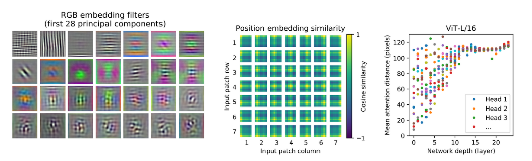
- 왼쪽: embedding filter을 시각화한 결과→ 많은 데이터를 pre-training하면, embedding filter가 CNN filter와 비슷한 기능을 보임
- 가운데: position embedding을 시각화한 결과→ 각각의 위치를 잘 학습함 (노란색 부분 확인 ex 가운데 부분은 가운데에 노란색으로, 아래쪽으로 갈수록 아래에 노란색이 존재)
- 오른쪽: 낮은 layer에서는 CNN의 낮은 layer처럼 각각의 이미지를 나타냄→ 마지막으로 갈수록 이미지의 통합적인 모습을 나타냄
'Deep Learning > [논문] Paper Review' 카테고리의 다른 글
| U-Net (0) | 2023.07.05 |
|---|---|
| Bert (0) | 2023.07.05 |
| RetinaNet (0) | 2023.07.05 |
| GPT-1 (0) | 2023.07.05 |
| DeepLab V2: Semantic Image Segmentation with Convolutional Nets, Atrous Convolution and Fully Connected CRFs (0) | 2023.07.05 |


