0. Abstract

Figure 1: Given any two unordered image collections X and Y , our algorithm learns to automatically “translate” an image from one into the other and vice versa: (left) Monet paintings and landscape photos from Flickr; (center) zebras and horses from ImageNet; (right) summer and winter Yosemite photos from Flickr. Example application (bottom): using a collection of paintings of famous artists, our method learns to render natural photographs into the respective styles.
그림 1: 임의의 두 개의 이미지 집합 X와 Y가 주어졌을 때, 우리의 알고리즘은 한 이미지를 다른 이미지로 "변환"하고 그 반대로 수행하는 방법을 자동으로 학습합니다. (왼쪽) Monet의 그림과 Flickr의 풍경 사진; (가운데) ImageNet의 얼룩말과 말; (오른쪽) Flickr의 여름과 겨울 요세미티 사진입니다. 예제 응용 (아래): 유명한 예술가들의 그림 컬렉션을 사용하여 우리의 방법은 자연 사진을 해당 스타일로 렌더링하는 방법을 학습합니다.
Image-to-image translation is a class of vision and graphics problems where the goal is to learn the mapping between an input image and an output image using a training set of aligned image pairs. However, for many tasks, paired training data will not be available. We present an approach for learning to translate an image from a source domain X to a target domain Y in the absence of paired examples. Our goal is to learn a mapping G : X → Y such that the distribution of images from G(X) is indistinguishable from the distribution Y using an adversarial loss. Because this mapping is highly under-constrained, we couple it with an inverse mapping F : Y → X and introduce a cycle consistency loss to enforce F(G(X)) ≈ X (and vice versa). Qualitative results are presented on several tasks where paired training data does not exist, including collection style transfer, object transfiguration, season transfer, photo enhancement, etc. Quantitative comparisons against several prior methods demonstrate the superiority of our approach.
이미지 간 변환은 입력 이미지와 출력 이미지 사이의 매핑을 학습하는 비전 및 그래픽스 문제의 한 유형입니다. 일치된 이미지 쌍의 학습 세트를 사용하여 입력 이미지와 출력 이미지 간의 매핑을 학습하는 것이 목표입니다. 그러나 많은 작업에서는 쌍으로 이루어진 훈련 데이터를 사용할 수 없습니다. 우리는 짝지어진 예제가 없을 때 소스 도메인 X에서 대상 도메인 Y로 이미지를 변환하는 방법을 제시합니다. 우리의 목표는 G: X → Y라는 매핑을 학습하는 것인데, 이때 G(X)의 이미지 분포가 적대적 손실을 사용하여 분포 Y와 구별할 수 없도록 합니다. 이러한 매핑은 매우 불충분한 제약을 가지고 있으므로 역 매핑 F: Y → X와 함께 결합하고 F(G(X)) ≈ X (반대의 경우도 마찬가지)를 강제하기 위해 사이클 일관성 손실을 도입합니다. 짝지어진 훈련 데이터가 없는 여러 작업에 대한 질적인 결과를 제시하며, 컬렉션 스타일 변환, 객체 변형, 계절 변환, 사진 개선 등을 포함합니다. 기존 방법과의 양적 비교는 우리의 접근 방식의 우수성을 입증합니다.
1. Introduction

Figure 2: Paired training data (left) consists of training examples {xi , yi} N i=1, where the correspondence between xi and yi exists [22]. We instead consider unpaired training data (right), consisting of a source set {xi} N i=1 (xi ∈ X) and a target set {yj}M j=1 (yj ∈ Y ), with no information provided as to which xi matches which yj . Figure 2: 매칭된 훈련 데이터 (왼쪽)는 훈련 예시 {xi, yi} N i=1로 구성되며, xi와 yi 사이의 대응이 존재합니다 [22]. 반면에 우리는 매칭되지 않은 훈련 데이터 (오른쪽)를 고려합니다. 이는 소스 집합 {xi} N i=1 (xi ∈ X)와 타겟 집합 {yj}M j=1 (yj ∈ Y)로 구성되며, 어떤 xi가 어떤 yj와 일치하는지에 대한 정보가 제공되지 않습니다.
What did Claude Monet see as he placed his easel by the bank of the Seine near Argenteuil on a lovely spring day in 1873 (Figure 1, top-left)? A color photograph, had it been invented, may have documented a crisp blue sky and a glassy river reflecting it. Monet conveyed his impression of this same scene through wispy brush strokes and a bright palette.

What if Monet had happened upon the little harbor in Cassis on a cool summer evening (Figure 1, bottom-left)? A brief stroll through a gallery of Monet paintings makes it possible to imagine how he would have rendered the scene: perhaps in pastel shades, with abrupt dabs of paint, and a somewhat flattened dynamic range. We can imagine all this despite never having seen a side by side example of a Monet painting next to a photo of the scene he painted. Instead, we have knowledge of the set of Monet paintings and of the set of landscape photographs. We can reason about the stylistic differences between thesetwo sets, and thereby imagine what a scene might look like if we were to “translate” it from one set into the other.
1873년 봄, 클로드 모네가 아르장튤 인근 세느 강 둑 옆에 이지를 세우고 있을 때 (Figure 1, 왼쪽 상단), 그는 어떤 풍경을 보았을까요? 만약 컬러 사진이 이미 발명되어 있다면, 청명한 파란 하늘과 그것을 반영하는 유리처럼 맑은 강이 사진에 담겨있을 수도 있었습니다. 모네는 이 같은 장면을 얇은 붓질과 밝은 팔레트를 통해 자신의 인상을 전달했습니다. 만약 모네가 캐시스의 작은 항구에서 서늘한 여름 저녁에 그곳을 발견했다면 (Figure 1, 왼쪽 하단), 모네의 그림 갤러리를 잠시 돌아보면 그가 어떻게 그 장면을 표현했을지 상상할 수 있습니다. 아마도 옅은 색조로, 갑작스러운 털기로, 약간 펼쳐진 다이내믹 레인지로 표현했을 것입니다.
우리는 이 모든 것을 모네의 그림과 그가 그린 장면의 사진을 나란히 본 적이 없어도 상상할 수 있습니다. 대신, 우리는 모네의 그림 모음과 풍경 사진 모음에 대한 지식을 가지고 있습니다. 이 두 집합 간의 스타일적 차이를 추론할 수 있으며, 따라서 한 집합에서 다른 집합으로 "번역"한다면 장면이 어떻게 보일지 상상할 수 있습니다.
In this paper, we present a method that can learn to do the same: capturing special characteristics of one image collection and figuring out how these characteristics could be translated into the other image collection, all in the absence of any paired training examples. This problem can be more broadly described as imageto-image translation [22], converting an image from one representation of a given scene, x, to another, y, e.g., grayscale to color, image to semantic labels, edge-map to photograph. Years of research in computer vision, image processing, computational photography, and graphics have produced powerful translation systems in the supervised setting, where example image pairs {xi , yi} N i=1 are available (Figure 2, left), e.g., [11, 19, 22, 23, 28, 33, 45, 56, 58, 62]. However, obtaining paired training data can be difficult and expensive. For example, only a couple of datasets exist for tasks like semantic segmentation (e.g., [4]), and they are relatively small. Obtaining input-output pairs for graphics tasks like artistic stylization can be even more difficult since the desired output is highly complex, typically requiring artistic authoring. For many tasks, like object transfiguration (e.g., zebra↔horse, Figure 1 top-middle), the desired output is not even well-defined.
이 논문에서는 어떤 이미지 모음의 특징을 포착하고 이러한 특징을 다른 이미지 모음으로 어떻게 변환할 수 있는지 학습하는 방법을 제안합니다. 이는 어떠한 대응되는 훈련 예시도 없는 상황에서 이루어지는 것입니다. 이 문제는 이미지 간 변환, 예를 들어 그레이스케일에서 컬러로, 이미지에서 시맨틱 레이블로, 엣지 맵에서 사진으로의 변환 등으로 더 넓게 설명될 수 있습니다. 컴퓨터 비전, 이미지 처리, 계산 사진술 및 그래픽스 분야에서 수년간의 연구로는 예시 이미지 쌍 {xi, yi} N i=1 이 제공되는 지도 학습 환경에서 강력한 변환 시스템을 개발했습니다(Figure 2, 왼쪽), 예를 들면 [11, 19, 22, 23, 28, 33, 45, 56, 58, 62] 등이 있습니다.
그러나 대응되는 훈련 데이터를 얻는 것은 어렵고 비용이 많이 들 수 있습니다. 예를 들어 시맨틱 분할과 같은 작업에는 몇 개의 데이터셋만 존재하며 상대적으로 작습니다([4] 등). 예술적인 스타일화와 같은 그래픽 작업에 대해 입력-출력 쌍을 얻는 것은 더욱 어려울 수 있습니다. 원하는 출력은 매우 복잡하며 일반적으로 예술적 저작을 필요로 합니다. 얼룩말 ↔ 말과 같은 객체 변형과 같은 많은 작업에서는 원하는 출력이 명확하게 정의되지 않을 수도 있습니다.
We therefore seek an algorithm that can learn to translate between domains without paired input-output examples (Figure 2, right). We assume there is some underlying relationship between the domains – for example, that they are two different renderings of the same underlying scene – and seek to learn that relationship. Although we lack supervision in the form of paired examples, we can exploit supervision at the level of sets: we are given one set of images in domain X and a different set in domain Y . We may train a mapping G : X → Y such that the output yˆ = G(x), x ∈ X, is indistinguishable from images y ∈ Y by an adversary trained to classify yˆ apart from y. In theory, this objective can induce an output distribution over yˆ that matches the empirical distribution pdata(y) (in general, this requires G to be stochastic) [16]. The optimal G thereby translates the domain X to a domain Yˆ distributed identically to Y . However, such a translation does not guarantee that an individual input x and output y are paired up in a meaningful way – there are infinitely many mappings G that will induce the same distribution over yˆ. Moreover, in practice, we have found it difficult to optimize the adversarial objective in isolation: standard procedures often lead to the wellknown problem of mode collapse, where all input images map to the same output image and the optimization fails to make progress [15].
따라서, 우리는 입력-출력 쌍의 예시 없이 도메인 간에 번역을 학습할 수 있는 알고리즘을 찾고 있습니다(Figure 2, 오른쪽). 우리는 도메인 간에
어떤 기저 신경을 가진 관계가 있다고 가정하고 그 관계를 학습하려고 합니다. 예시 쌍 형태로는 지도 학습의 감독이 부족하지만, 우리는 집합 수준에서의 감독을 활용할 수 있습니다: 우리에게는 도메인 X의 이미지 집합과 도메인 Y의 다른 이미지 집합이 주어집니다. 우리는 매핑 G: X → Y를 학습시켜서 출력 yˆ = G(x), x ∈ X가 y ∈ Y 이미지와 차별화되지 않도록 할 수 있습니다. 이를 위해 yˆ와 y를 분류하는 데에 훈련된 적대적인 모델을 사용합니다. 이론적으로, 이 목표는 yˆ에 대한 출력 분포를 경험적 분포 pdata(y)와 일치시킬 수 있습니다 (일반적으로 이를 위해서는 G가 확률적이어야 함) [16]. 따라서 최적의 G는 도메인 X를 도메인 Yˆ로 번역하며, Y와 동일하게 분포됩니다.
그러나 이러한 번역은 개별적인 입력 x와 출력 y가 의미 있는 방식으로 대응된다는 것을 보장하지 않습니다 - yˆ에 대해 동일한 분포를 유도하는 무한히 많은 매핑 G가 존재할 수 있습니다.게다가 실제로는 적대적 목적을 독립적으로 최적화하기가 어려운 것으로 판명되었습니다. 표준 절차는 종종 모드 붕괴라고 알려진 문제에 이르게 되는데,
이는 모든 입력 이미지가 동일한 출력 이미지로 매핑되고 최적화가 진전되지 않는 문제입니다 [15].These issues call for adding more structure to our objective. Therefore, we exploit the property that translation should be “cycle consistent”, in the sense that if we translate, e.g., a sentence from English to French, and then translate it back from French to English, we should arrive back at the original sentence [3]. Mathematically, if we have a translator G : X → Y and another translator F : Y → X, then G and F should be inverses of each other, and both mappings should be bijections. We apply this structural assumption by training both the mapping G and F simultaneously, and adding a cycle consistency loss [64] that encourages F(G(x)) ≈ x and G(F(y)) ≈ y. Combining this loss with adversarial losses on domains X and Y yields our full objective for unpaired image-to-image translation. We apply our method to a wide range of applications, including collection style transfer, object transfiguration, season transfer and photo enhancement. We also compare against previous approaches that rely either on hand-defined factorizations of style and content, or on shared embedding functions, and show that our method outperforms these baselines. We provide both PyTorch and Torch implementations. Check out more results at our website. 이러한 문제들은
목적에 더 많은 구조를 추가할 필요가 있다는 것을 시사합니다. 따라서, 우리는 번역은 "cycle consistent" 해야 한다는 속성을 활용합니다. 즉, 예를 들어 영어에서 프랑스어로 문장을 번역하고 다시 프랑스어에서 영어로 번역하면 원래의 문장으로 돌아와야 합니다 [3]. 수학적으로, 만약 우리에게 G: X → Y 번역기와 F: Y → X 번역기가 있다면, G와 F는 서로의 역함수여야 하며 두 매핑은 전단사 함수(bijection)이어야 합니다. 우리는 이 구조적 가정을 적용하기 위해 매핑 G와 F를 동시에 학습하고, F(G(x)) ≈ x와 G(F(y)) ≈ y를 장려하는 cycle consistency loss [64]를 추가합니다. X와 Y 도메인에서의 적대적 손실과 이 손실을 결합하여 unpaired 이미지 간 번역을 위한 완전한 목적을 얻습니다.
우리의 방법을 컬렉션 스타일 전이, 객체 변형, 계절 전이 및 사진 개선 등 다양한 응용 분야에 적용합니다. 또한, 스타일과 콘텐츠의 수동 정의된 요소 분해나 공유된 임베딩 함수에 의존하는 이전 접근 방식과 비교하고, 우리의 방법이 이러한 기준 모델을 능가한다는 것을 보여줍니다. 우리는 PyTorch와 Torch 구현을 제공합니다. 자세한 결과는 우리의 웹사이트를 확인해주세요.
2. Related Work

Figure 3: (a) Our model contains two mapping functions G : X → Y and F : Y → X, and associated adversarial discriminators DY and DX. DY encourages G to translate X into outputs indistinguishable from domain Y , and vice versa for DX and F. To further regularize the mappings, we introduce two cycle consistency losses that capture the intuition that if we translate from one domain to the other and back again we should arrive at where we started: (b) forward cycle-consistency loss: x → G(x) → F(G(x)) ≈ x, and (c) backward cycle-consistency loss: y → F(y) → G(F(y)) ≈ y Figure 3: (a) 우리의 모델은 두 개의 매핑 함수 G: X → Y와 F: Y → X를 포함하고 있으며, 이에 연결된 적대적 판별자 DY와 DX가 있습니다. DY는 G가 X를 Y 도메인과 구별할 수 없는 출력으로 번역하도록 장려하며, DX와 F에 대해서도 마찬가지입니다. 매핑을 더욱 규제하기 위해, 우리는 두 개의 순환 일관성 손실을 도입합니다. 이 손실은 한 도메인에서 다른 도메인으로 번역한 다음 다시 되돌아오면 원래의 위치로 도달해야 한다는 직관을 포착합니다: (b) 순방향 순환 일관성 손실: x → G(x) → F(G(x)) ≈ x, 그리고 (c) 역방향 순환 일관성 손실: y → F(y) → G(F(y)) ≈ y
Generative Adversarial Networks (GANs)
[16, 63] have achieved impressive results in image generation [6, 39], image editing [66], and representation learning [39, 43, 37]. Recent methods adopt the same idea for conditional image generation applications, such as text2image [41], image inpainting [38], and future prediction [36], as well as to other domains like videos [54] and 3D data [57]. The key to GANs’ success is the idea of an adversarial loss that forces the generated images to be, in principle, indistinguishable from real photos. This loss is particularly powerful for image generation tasks, as this is exactly the objective that much of computer graphics aims to optimize. We adopt an adversarial loss to learn the mapping such that the translated images cannot be distinguished from images in the target domain.
생성적 적대 신경망(GANs)은 이미지 생성, 이미지 편집 및 표현 학습과 같은 이미지 관련 작업에서 인상적인 결과를 달성했습니다 [6, 39, 66]. 최근의 방법들은 이 아이디어를 텍스트에서 이미지로의 조건부 이미지 생성, 이미지 보정, 미래 예측과 같은 응용 프로그램뿐만 아니라 비디오 [54] 및 3D 데이터 [57]와 같은 다른 도메인에도 동일하게 적용합니다. GAN의 성공의 핵심은 생성된 이미지가 원칙적으로 실제 사진과 구별할 수 없도록 하는 적대적 손실의 개념입니다. 이 손실은 이미지 생성 작업에 대해 매우 강력하며, 이것이 컴퓨터 그래픽스의 주요 목표입니다. 우리는 적대적 손실을 채택하여 변환된 이미지가 대상 도메인의 이미지와 구별할 수 없도록 매핑을 학습합니다. Image-to-Image Translation
The idea of image-toimage translation goes back at least to Hertzmann et al.’s Image Analogies [19], who employ a non-parametric texture model [10] on a single input-output training image pair. More recent approaches use a dataset of input-output examples to learn a parametric translation function using CNNs (e.g., [33]). Our approach builds on the “pix2pix” framework of Isola et al. [22], which uses a conditional generative adversarial network [16] to learn a mapping from input to output images. Similar ideas have been applied to various tasks such as generating photographs from sketches [44] or from attribute and semantic layouts [25]. However, unlike the above prior work, we learn the mapping without paired training examples. 이미지 대 이미지 변환은 적어도 Hertzmann et al.의 Image Analogies [19]에서 시작된 아이디어로, 단일 입력-출력 훈련 이미지 쌍에 비파라미터 텍스처 모델 [10]을 사용합니다. 최근의 접근 방식은 입력-출력 예제 데이터셋을 사용하여 CNN을 사용하여 매개변수화된 변환 함수를 학습합니다 (예: [33]). 우리의 접근 방식은 Isola et al.의 "pix2pix" 프레임워크 [22]를 기반으로 합니다. 이 프레임워크는 조건부 생성적 적대 신경망 [16]을 사용하여 입력 이미지에서 출력 이미지로의 매핑을 학습합니다. 비슷한 아이디어가 스케치에서 사진 또는 속성 및 의미적 레이아웃에서 사진을 생성하는 등 다양한 작업에 적용되었습니다 [44, 25]. 하지만, 이전의 작업과 달리 우리는 페어링된 훈련 예제 없이 매핑을 학습합니다.
Unpaired Image-to-Image Translation
Several other methods also tackle the unpaired setting, where the goal is to relate two data domains: X and Y . Rosales et al. [42] propose a Bayesian framework that includes a prior based on a patch-based Markov random field computed from a source image and a likelihood term obtained from multiple style images. More recently, CoGAN [32] and cross-modal scene networks [1] use a weight-sharing strategy to learn a common representation across domains. Concurrent to our method, Liu et al. [31] extends the above framework with a combination of variational autoencoders [27] and generative adversarial networks [16]. Another line of concurrent work [46, 49, 2] encourages the input and output to share specific “content” features even though they may differ in “style“. These methods also use adversarial networks, with additional terms to enforce the output to be close to the input in a predefined metric space, such as class label space [2], image pixel space [46], and image feature space [49]. Unlike the above approaches, our formulation does not rely on any task-specific, predefined similarity function be tween the input and output, nor do we assume that the input and output have to lie in the same low-dimensional embedding space. This makes our method a general-purpose solution for many vision and graphics tasks. We directly compare against several prior and contemporary approaches in Section 5.1. 쌍이 아닌(unpaired) 이미지 대 이미지 변환에는 다른 몇 가지 방법들도 있습니다. 여기서 목표는 X와 Y라는 두 데이터 도메인을 관련시키는 것입니다. Rosales 등 [42]은 소스 이미지로부터 계산된 패치 기반 마르코프 랜덤 필드를 기반으로 한 사진과 여러 스타일 이미지에서 얻은 가능도 항을 포함하는 베이지안 프레임워크를 제안합니다. 최근에는 CoGAN [32]과 교차 모달(scene) 네트워크 [1]가 도메인 간에 공통 표현을 학습하기 위해 가중치 공유 전략을 사용합니다. 우리의 방법과 동시에, Liu 등 [31]은 변이형 오토인코더 [27]와 생성적 적대 신경망 [16]의 조합으로 위의 프레임워크를 확장합니다. 동시에 다른 방법 [46, 49, 2]은 "콘텐츠(content)" 특징을 공유하도록 입력과 출력을 장려하지만 "스타일(style)"은 다를 수 있도록 합니다. 이러한 방법들도 적대적 신경망을 사용하며, 추가적인 항들을 사용하여 출력이 미리 정의된 메트릭 공간(예: 클래스 레이블 공간 [2], 이미지 픽셀 공간 [46], 이미지 특징 공간 [49])에서 입력에 가까워지도록 합니다. 위의 접근 방식과 달리, 우리의 방식은 입력과 출력 사이에 작업 특정 사전 정의된 유사도 함수에 의존하지 않으며, 또한 입력과 출력이 동일한 저차원 임베딩 공간에 있어야 한다고 가정하지 않습니다. 이로써 우리의 방법은 많은 비전 및 그래픽 작업에 대한 범용적인 솔루션으로 사용될 수 있습니다. 5.1절에서 이전의 몇 가지 방법과 현대적인 방법들과 직접 비교합니다.
Cycle Consistency
The idea of using transitivity as a way to regularize structured data has a long history. In visual tracking, enforcing simple forward-backward consistency has been a standard trick for decades [24, 48]. In the language domain, verifying and improving translations via “back translation and reconciliation” is a technique used by human translators [3] (including, humorously, by Mark Twain [51]), as well as by machines [17]. More recently, higher-order cycle consistency has been used in structure from motion [61], 3D shape matching [21], cosegmentation [55], dense semantic alignment [65, 64], and depth estimation [14]. Of these, Zhou et al. [64] and Godard et al. [14] are most similar to our work, as they use a cycle consistency loss as a way of using transitivity to supervise CNN training. In this work, we are introducing a similar loss to push G and F to be consistent with each other. Concurrent with our work, in these same proceedings, Yi et al. [59] independently use a similar objective for unpaired image-to-image translation, inspired by dual learning in machine translation [17]. 환형 일관성 (Cycle Consistency)은 구조화된 데이터를 규제하는 방법으로서 오랜 역사를 가지고 있습니다. 시각 추적에서는 간단한 순방향-역방향 일관성을 강제하는 것이 수십 년간 표준적인 기법으로 사용되었습니다 [24, 48]. 언어 분야에서는 인간 번역가들이 [3] (Mark Twain도 재미있게 언급한) 백 번역과 조정을 통해 번역을 확인하고 개선하는 기술을 사용하며, 기계 번역에서도 이러한 방식을 적용합니다 [17]. 최근에는 공간 구조 추론 [61], 3D 형상 매칭 [21], 공유 분할 [55], 밀집 시맨틱 정렬 [65, 64], 깊이 추정 [14] 등에서 고차 환형 일관성이 사용되었습니다. 이 중에서도 Zhou 등 [64]과 Godard 등 [14]는 우리의 작업과 가장 유사하며, 이들은 환형 일관성 손실을 사용하여 전이성을 이용하여 CNN 학습을 감독합니다. 본 논문에서는 G와 F가 서로 일관되도록 하는 유사한 손실을 도입합니다. 동시에, 같은 논문에서는 Yi 등 [59]이 기계 번역의 이중 학습에서 영감을 받아 비슷한 목적을 위해 독립적으로 비슷한 목표를 사용합니다 [17].
Neural Style Transfer
[13, 23, 52, 12] is another way to perform image-to-image translation, which synthesizes a novel image by combining the content of one image with the style of another image (typically a painting) based on matching the Gram matrix statistics of pre-trained deep features. Our primary focus, on the other hand, is learning the mapping between two image collections, rather than between two specific images, by trying to capture correspondences between higher-level appearance structures. Therefore, our method can be applied to other tasks, such as painting→ photo, object transfiguration, etc. where single sample transfer methods do not perform well. We compare these two methods in Section 5.2. 신경 스타일 전이 (Neural Style Transfer) [13, 23, 52, 12]은 이미지 간 전환을 수행하는 또 다른 방법으로, 사전에 훈련된 깊은 특징의 Gram 행렬 통계를 매칭하여 한 이미지의 콘텐츠와 다른 이미지(일반적으로 그림)의 스타일을 결합하여 새로운 이미지를 합성합니다. 그러나 저희의 주요 관심은 두 개의 이미지 컬렉션 간의 매핑을 학습하는 것이며, 특정 이미지 간의 전환보다는 더 높은 수준의 외관 구조 간의 대응을 포착하려는 것입니다. 따라서 저희의 방법은 화가 → 사진, 물체 변형 등과 같은 단일 샘플 전환 방법이 잘 작동하지 않는 다른 작업에도 적용할 수 있습니다. 이러한 두 가지 방법을 5.2절에서 비교합니다.
3. Formulation

Figure 4: The input images x, output images G(x) and the reconstructed images F(G(x)) from various experiments. From top to bottom: photo↔Cezanne, horses↔zebras, winter→summer Yosemite, aerial photos↔Google maps Figure 4: 다양한 실험에서의 입력 이미지 x, 출력 이미지 G(x), 그리고 재구성된 이미지 F(G(x))입니다. 위에서 아래로: 사진↔세잔, 말↔얼룩말, 겨울→여름 요세미티, 항공 사진↔구글 지도
Our goal is to learn mapping functions between two domains X and Y given training samples {xi} N i=1 where xi ∈ X and {yj}M j=1 where yj ∈ Y 1 . We denote the data distribution as x ∼ pdata(x) and y ∼ pdata(y). As illustrated in Figure 3 (a), our model includes two mappings G : X → Y and F : Y → X. In addition, we introduce two adversarial discriminators DX and DY , where DX aims to distinguish between images {x} and translated images {F(y)}; in the same way, DY aims to discriminate between {y} and {G(x)}. Our objective contains two types of terms: adversarial losses [16] for matching the distribution of generated images to the data distribution in the target domain; and cycle consistency losses to prevent the learned mappings G and F from contradicting each other.
우리의 목표는 훈련 샘플 {xi}N i=1 (여기서 xi ∈ X)와 {yj}M j=1 (여기서 yj ∈ Y)이 주어진 두 도메인 X와 Y 사이의 매핑 함수를 학습하는 것입니다. 데이터 분포는 x ∼ pdata(x)와 y ∼ pdata(y)로 표기됩니다. Figure 3 (a)에 나와 있는 것처럼, 우리의 모델에는 두 개의 매핑 G: X → Y와 F: Y → X가 포함되어 있습니다. 추가로, 우리는 DX와 DY라는 두 개의 적대적 판별자를 소개합니다. DX는 이미지 집합 {x}와 변환된 이미지 집합 {F(y)} 사이를 구별하려고 하며, 마찬가지로 DY는 {y}와 {G(x)} 사이를 구별하려고 합니다. 우리의 목적은 두 가지 유형의 항목으로 구성되어 있습니다: 생성된 이미지의 분포를 대상 도메인의 데이터 분포와 일치시키기 위한 적대적 손실 [16] 및 학습된 매핑 G와 F가 서로 모순되지 않도록 하기 위한 사이클 일관성 손실입니다.
3.1. Adversarial Loss
We apply adversarial losses [16] to both mapping functions. For the mapping function G : X → Y and its discriminator DY , we express the objective as: LGAN(G, DY , X, Y ) = Ey∼pdata(y) [log DY (y)] + Ex∼pdata(x) [log(1 − DY (G(x))], (1) where G tries to generate images G(x) that look similar to images from domain Y , while DY aims to distinguish between translated samples G(x) and real samples y. G aims to minimize this objective against an adversary D that tries to maximize it, i.e., minG maxDY LGAN(G, DY , X, Y ). We introduce a similar adversarial loss for the mapping function F : Y → X and its discriminator DX as well: i.e., minF maxDX LGAN(F, DX, Y, X).
3.1. 적대적 손실
우리는 두 개의 매핑 함수에 적대적 손실 [16]을 적용합니다. 매핑 함수 G : X → Y와 그 판별자 DY에 대해, 우리는 다음과 같이 목적 함수를 표현합니다: LGAN(G, DY , X, Y ) = Ey∼pdata(y) [log DY (y)] + Ex∼pdata(x) [log(1 − DY (G(x))], (1)
여기서 G는 도메인 Y의 이미지와 유사한 이미지 G(x)를 생성하려고 하며, DY는 번역된 샘플 G(x)과 실제 샘플 y를 구별하려고 합니다. G는 적대적인 상대인 D가 이 목적 함수를 최대화하려고 할 때 이를 최소화하려고 합니다. 즉, minG maxDY LGAN(G, DY , X, Y)를 목표로 합니다. 우리는 매핑 함수 F : Y → X와 그 판별자 DX에 대해서도 유사한 적대적 손실을 도입합니다: minF maxDX LGAN(F, DX, Y, X).
3.2. Cycle Consistency Loss
Adversarial training can, in theory, learn mappings G and F that produce outputs identically distributed as target domains Y and X respectively (strictly speaking, this requires G and F to be stochastic functions) [15]. However, with large enough capacity, a network can map the same set of input images to any random permutation of images in the target domain, where any of the learned mappings can induce an output distribution that matches the target distribution. Thus, adversarial losses alone cannot guarantee that the learned function can map an individual input xi to a desired output yi . To further reduce the space of possible mapping functions, we argue that the learned mapping functions should be cycle-consistent: as shown in Figure 3 (b), for each image x from domain X, the image translation cycle should be able to bring x back to the original image, i.e., x → G(x) → F(G(x)) ≈ x. We call this forward cycle consistency. Similarly, as illustrated in Figure 3 (c), for each image y from domain Y , G and F should also satisfy backward cycle consistency: y → F(y) → G(F(y)) ≈ y. We incentivize this behavior using a cycle consistency loss: Lcyc(G, F) = Ex∼pdata(x) [kF(G(x)) − xk1] + Ey∼pdata(y) [kG(F(y)) − yk1]. (2)
3.2. 순환 일관성 손실
이론적으로 적대적 훈련은 매핑 함수 G와 F가 각각 대상 도메인 Y와 X로부터 동일한 분포를 갖는 출력을 생성하도록 학습할 수 있습니다 (엄밀히 말하면, 이를 위해서는 G와 F가 확률적인 함수이어야 함) [15]. 그러나 충분한 용량을 가진 네트워크는 입력 이미지의 동일한 집합을 대상 도메인의 이미지의 임의의 순열로 매핑할 수 있습니다. 이때 학습된 매핑 중 어떤 것이든 대상 분포와 일치하는 출력 분포를 유도할 수 있습니다. 따라서 적대적 손실만으로는 학습된 함수가 개별 입력 xi를 원하는 출력 yi로 매핑할 수 있는지를 보장할 수 없습니다. 가능한 매핑 함수의 공간을 더욱 줄이기 위해, 학습된 매핑 함수들은 순환 일관성을 가져야 한다고 주장합니다. Figure 3 (b)에 나와 있는 것처럼 도메인 X의 각 이미지 x에 대해 이미지 변환 순환은 x를 원래의 이미지로 되돌릴 수 있어야 합니다. 즉, x → G(x) → F(G(x)) ≈ x가 되어야 합니다. 이를 순방향 순환 일관성이라고 합니다. 마찬가지로 Figure 3 (c)에서 보여지듯이 도메인 Y의 각 이미지 y에 대해서도 G와 F는 역방향 순환 일관성을 만족해야 합니다: y → F(y) → G(F(y)) ≈ y. 이러한 동작을 장려하기 위해 순환 일관성 손실을 도입합니다: Lcyc(G, F) = Ex∼pdata(x) [kF(G(x)) − xk1] + Ey∼pdata(y) [kG(F(y)) − yk1]. (2)
In preliminary experiments, we also tried replacing the L1 norm in this loss with an adversarial loss between F(G(x)) and x, and between G(F(y)) and y, but did not observe improved performance.
The behavior induced by the cycle consistency loss can be observed in Figure 4: the reconstructed images F(G(x)) end up matching closely to the input images x.
예비 실험에서는 이 손실의 L1 노름을 F(G(x))와 x, G(F(y))와 y 간의 적대적 손실로 대체해 보았지만 개선된 성능을 관찰하지 못했습니다.
순환 일관성 손실에 의해 유도되는 동작은 Figure 4에서 관찰할 수 있습니다: 재구성된 이미지 F(G(x))는 입력 이미지 x와 근접하게 일치합니다.
3.3. Full Objective
Our full objective is: L(G, F, DX, DY ) =LGAN(G, DY , X, Y ) + LGAN(F, DX, Y, X) + λLcyc(G, F), where λ controls the relative importance of the two objectives. We aim to solve: G ∗ , F∗ = arg min G,F max Dx,DY L(G, F, DX, DY ). (4) Notice that our model can be viewed as training two “autoencoders” [20]: we learn one autoencoder F ◦ G : X → X jointly with another G◦F : Y → Y . However, these autoencoders each have special internal structures: they map an image to itself via an intermediate representation that is a translation of the image into another domain. Such a setup can also be seen as a special case of “adversarial autoencoders” [34], which use an adversarial loss to train the bottleneck layer of an autoencoder to match an arbitrary target distribution. In our case, the target distribution for the X → X autoencoder is that of the domain Y .
저희의 전체 목적은 다음과 같습니다: L(G, F, DX, DY ) = LGAN(G, DY , X, Y ) + LGAN(F, DX, Y, X) + λLcyc(G, F), 여기서 λ는 두 목적의 상대적 중요도를 조절합니다. 저희는 다음을 해결하기 위해 노력합니다: G ∗ , F∗ = arg min G,F max Dx,DY L(G, F, DX, DY ). (4) 저희 모델은 두 개의 "자동 인코더" [20]를 학습하는 것으로 볼 수 있습니다: 하나는 F ◦ G : X → X 자동 인코더이고, 다른 하나는 G◦F : Y → Y 자동 인코더입니다. 그러나 이러한 자동 인코더는 각각 특별한 내부 구조를 가지고 있습니다: 이미지를 중간 표현으로 변환하여 자신 자신에게 매핑합니다. 이러한 설정은 "적대적 자동 인코더" [34]의 특수한 경우로도 볼 수 있습니다. 이 경우, X → X 자동 인코더의 대상 분포는 도메인 Y의 분포와 일치하도록 자동 인코더의 병목 계층을 적대적 손실로 학습합니다.
In Section 5.1.4, we compare our method against ablations of the full objective, including the adversarial loss LGAN alone and the cycle consistency loss Lcyc alone, and empirically show that both objectives play critical roles in arriving at high-quality results. We also evaluate our method with only cycle loss in one direction and show that a single cycle is not sufficient to regularize the training for this under-constrained problem.
5.1.4절에서는 우리의 방법을 전체 목적과 비교하여 검토하며, 단독으로 사용되는 적대적 손실 LGAN과 순환 일관성 손실 Lcyc를 포함한 추론에 대해 비교합니다. 우리는 실험적으로 이 두 가지 목적이 모두 고화질 결과에 중요한 역할을 하는 것을 입증합니다. 또한 단일 방향의 순환 손실만 사용하여 우리의 방법을 평가하고, 이렇게 하면 이런 미정의 문제에 대한 훈련을 규제하기에는 단일 순환만으로는 충분하지 않음을 보여줍니다.
4. Implementation
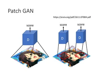
4.1 Network Architecture We adopt the architecture for our generative networks from Johnson et al. [23] who have shown impressive results for neural style transfer and superresolution. This network contains three convolutions, several residual blocks [18], two fractionally-strided convolutions with stride 1 2 , and one convolution that maps features to RGB. We use 6 blocks for 128 × 128 images and 9 blocks for 256×256 and higher-resolution training images. Similar to Johnson et al. [23], we use instance normalization [53]. For the discriminator networks we use 70 × 70 PatchGANs [22, 30, 29], which aim to classify whether 70 × 70 overlapping image patches are real or fake. Such a patch-level discriminator architecture has fewer parameters than a full-image discriminator and can work on arbitrarilysized images in a fully convolutional fashion [22]. 우리는 Johnson 등 [23]의 생성 네트워크 아키텍처를 채택했습니다. 이들은 신경 스타일 전송과 초해상도에 대해 인상적인 결과를 보여주었습니다. 이 네트워크는 세 개의 합성곱, 여러 개의 잔차 블록 [18], 스트라이드 1/2로 구성된 두 개의 분수 스트라이드 합성곱 및 특징을 RGB로 매핑하는 합성곱으로 구성됩니다. 우리는 128×128 이미지에 6개의 블록을 사용하고, 256×256 및 더 높은 해상도의 훈련 이미지에는 9개의 블록을 사용합니다. Johnson 등 [23]과 마찬가지로 인스턴스 정규화 [53]를 사용합니다. 판별자 네트워크에는 70×70 패치 단위 판별자인 PatchGAN [22, 30, 29]을 사용합니다. 이는 70×70 겹치는 이미지 패치가 실제인지 가짜인지를 분류하는 것을 목표로 합니다. 이러한 패치 수준의 판별자 아키텍처는 전체 이미지 판별자보다 매개변수가 적으며, 완전 컨볼루션 방식으로 임의 크기의 이미지에서 작동할 수 있습니다 [22].
4.2 Training details We apply two techniques from recent works to stabilize our model training procedure. First, for LGAN (Equation 1), we replace the negative log likelihood objective by a least-squares loss [35]. This loss is more stable during training and generates higher quality results. In particular, for a GAN loss LGAN(G, D, X, Y ), we train the G to minimize Ex∼pdata(x) [(D(G(x)) − 1)2 ] and train the D to minimize Ey∼pdata(y) [(D(y) − 1)2 ] + Ex∼pdata(x) [D(G(x))2 ]. Second, to reduce model oscillation [15], we follow Shrivastava et al.’s strategy [46] and update the discriminators using a history of generated images rather than the ones produced by the latest generators. We keep an image buffer that stores the 50 previously created images. For all the experiments, we set λ = 10 in Equation 3. We use the Adam solver [26] with a batch size of 1. All networks were trained from scratch with a learning rate of 0.0002. We keep the same learning rate for the first 100 epochs and linearly decay the rate to zero over the next 100 epochs. Please see the appendix (Section 7) for more details about the datasets, architectures, and training procedures. 저희는 최근 연구에서 모델 훈련 절차를 안정화하기 위해 두 가지 기법을 적용합니다. 첫째로, LGAN (식 1)에 대해 음의 로그 우도 목적을 최소 제곱 손실 [35]로 대체합니다. 이 손실은 훈련 중에 더 안정적이며 높은 품질의 결과를 생성합니다. 특히, GAN 손실 LGAN(G, D, X, Y)에 대해 G를 Ex∼pdata(x) [(D(G(x)) - 1)2]를 최소화하도록 훈련하고, D를 Ey∼pdata(y) [(D(y) - 1)2] + Ex∼pdata(x) [D(G(x))2]를 최소화하도록 훈련합니다.
둘째로, 모델 진동을 줄이기 위해 Shrivastava 등의 전략 [46]을 따라 판별자를 최신 생성자가 생성한 이미지 대신 이전에 생성된 이미지의 기록을 사용하여 업데이트합니다. 우리는 50개의 이전에 생성된 이미지를 저장하는 이미지 버퍼를 유지합니다. 모든 실험에서 식 3에서 λ = 10으로 설정합니다. 배치 크기가 1인 Adam 솔버 [26]를 사용합니다. 모든 네트워크는 학습률 0.0002로 처음부터 훈련되었습니다. 처음 100 epoch에 대해 동일한 학습률을 유지하고 다음 100 epoch 동안 학습률을 선형적으로 감소시켰습니다. 데이터셋, 아키텍처 및 훈련 절차에 대한 자세한 내용은 부록 (섹션 7)를 참조해주십시오.
5. Results
We first compare our approach against recent methods for unpaired image-to-image translation on paired datasets where ground truth input-output pairs are available for evaluation. We then study the importance of both the adversarial loss and the cycle consistency loss and compare our full method against several variants. Finally, we demonstrate the generality of our algorithm on a wide range of applications where paired data does not exist. For brevity, we refer to our method as CycleGAN. The PyTorch and Torch code, models, and full results can be found at our website.
우리는 먼저, 평가를 위해 입력-출력 쌍의 그라운드 트루스가 있는 페어 데이터셋에서 비짝지어진 이미지 간 변환에 대한 최근 방법들과 우리의 접근법을 비교합니다. 그런 다음, 적대적 손실과 사이클 일관성 손실의 중요성을 연구하고, 여러 가지 변형에 대해 우리의 전체 방법을 비교합니다. 마지막으로, 비짝지어진 데이터가 존재하지 않는 다양한 응용 분야에서 우리의 알고리즘의 일반성을 보여줍니다. 간결함을 위해, 우리의 방법을 CycleGAN이라고 지칭합니다. PyTorch와 Torch 코드, 모델, 그리고 전체 결과는 우리의 웹사이트에서 찾을 수 있습니다.
5.1. Evaluation Using the same evaluation datasets and metrics as “pix2pix” [22], we compare our method against several baselines both qualitatively and quantitatively. The tasks include semantic labels↔photo on the Cityscapes dataset [4], and map↔aerial photo on data scraped from Google Maps. We also perform ablation study on the full loss function.
5.1. 평가 "pix2pix" [22]와 동일한 평가 데이터셋과 평가 지표를 사용하여 우리의 방법을 여러 기준과 양적으로 비교합니다. 작업은 Cityscapes 데이터셋 [4]에서의 시맨틱 레이블↔사진 및 Google Maps에서 크롤링한 지도↔항공 사진 등을 포함합니다. 또한 전체 손실 함수에 대한 줄기 연구도 수행합니다.
5.1.1 Evaluation Metrics AMT perceptual studies On the map↔aerial photo task, we run “real vs fake” perceptual studies on Amazon Mechanical Turk (AMT) to assess the realism of our outputs. We follow the same perceptual study protocol from Isola et al. [22], except we only gather data from 25 participants per algorithm we tested. Participants were shown a sequence of pairs of images, one a real photo or map and one fake (generated by our algorithm or a baseline), and asked to click on the image they thought was real. The first 10 trials of each session were practice and feedback was given as to whether the participant’s response was correct or incorrect. The remaining 40 trials were used to assess the rate at which each algorithm fooled participants. Each session only tested a single algorithm, and participants were only allowed to complete a single session. The numbers we report here are not directly comparable to those in [22] as our ground truth images were processed slightly differently 2 and the participant pool we tested may be differently distributed from those tested in [22] (due to running the experiment at a different date and time). Therefore, our numbers should only be used to compare our current method against the baselines (which were run under identical conditions), rather than against [22].
5.1.1 평가 지표 AMT 인지 연구 지도↔항공 사진 작업에서 우리의 출력물의 현실성을 평가하기 위해 Amazon Mechanical Turk (AMT)에서 "실제 vs 가짜" 인지 연구를 진행했습니다. 우리는 Isola et al. [22]의 인지 연구 프로토콜을 따르되, 테스트한 각 알고리즘마다 25명의 참가자로부터 데이터를 수집했습니다. 참가자들은 실제 사진 또는 지도와 가짜 이미지 (우리의 알고리즘 또는 기준선에서 생성된)로 이루어진 이미지 쌍의 일련의 시퀀스를 보고 어떤 이미지가 실제인지 클릭하도록 요청받았습니다. 각 세션의 처음 10번은 연습이며 참가자의 응답이 올바른지 여부에 대한 피드백이 제공되었습니다. 나머지 40번은 각 알고리즘이 참가자를 속일 비율을 평가하는 데 사용되었습니다. 각 세션은 하나의 알고리즘만을 테스트하며, 참가자는 한 번의 세션만 완료할 수 있었습니다. 여기에서 보고하는 숫자는 [22]의 숫자와 직접적으로 비교할 수 없습니다. 우리의 Ground Truth 이미지는 약간 다르게 처리되었으며, 우리가 테스트한 참가자 집단은 [22]에서 테스트된 집단과 다른 분포일 수 있습니다 (실험을 다른 날짜와 시간에 진행했기 때문에). 따라서 우리의 숫자는 우리의 현재 방법을 기준선과 (동일한 조건에서 실행된) 비교하기 위해 사용되어야 하며, [22]와의 비교에는 사용되어서는 안 됩니다.
FCN score Although perceptual studies may be the gold standard for assessing graphical realism, we also seek an automatic quantitative measure that does not require human experiments. For this, we adopt the “FCN score” from [22], and use it to evaluate the Cityscapes labels→photo task. The FCN metric evaluates how interpretable the generated photos are according to an off-the-shelf semantic segmentation algorithm (the fully-convolutional network, FCN, from [33]). The FCN predicts a label map for a generated photo. This label map can then be compared against the input ground truth labels using standard semantic segmentation metrics described below. The intuition is that if we generate a photo from a label map of “car on the road”, then we have succeeded if the FCN applied to the generated photo detects “car on the road”. Semantic segmentation metrics To evaluate the performance of photo→labels, we use the standard metrics from the Cityscapes benchmark [4], including per-pixel accuracy, per-class accuracy, and mean class Intersection-Over-Union (Class IOU) [4].
FCN 점수 인지 연구는 그래픽적인 현실성을 평가하기 위한 금기적인 기준일 수 있지만, 인간 실험이 필요하지 않은 자동적인 양적 측정 방법도 필요합니다. 이를 위해 우리는 [22]의 "FCN 점수"를 채택하고 Cityscapes 라벨→사진 작업을 평가하는 데 사용합니다. FCN 점수는 오프 더 셀프 시맨틱 분할 알고리즘 (Fully Convolutional Network, FCN)을 통해 생성된 사진의 해석 가능성을 평가합니다. FCN은 생성된 사진에 대해 레이블 맵을 예측합니다. 이 레이블 맵은 입력된 그라운드 트루스 레이블과 표준 시맨틱 분할 지표를 사용하여 비교할 수 있습니다. 직관적으로, "도로 위의 차"라는 레이블 맵에서 사진을 생성한다면, 생성된 사진에 적용된 FCN이 "도로 위의 차"를 감지하는 경우 성공한 것입니다.
시맨틱 분할 지표 사진→레이블의 성능을 평가하기 위해 Cityscapes 벤치마크 [4]의 표준 지표를 사용합니다. 이에는 픽셀당 정확도 (per-pixel accuracy), 클래스별 정확도 (per-class accuracy), 클래스간 교차영역-연합 (Class IOU)의 평균 클래스 (mean class Intersection-Over-Union) 등이 포함됩니다.
<논문 리뷰>
1. Intro

- GAN은 입력에 대해 하나의 이미지만 생성한다는 특징을 지님.
- unpaired data는 x와 y가 매칭되어있지 않기 때문에, 어떠한 입력이미지가 들어왔을 때, 어떠한 정답 이미지가 만들어져야 하는지 모름.
- 즉, 매칭되는 y없이 단순히 입력 x의 특성을 도메인 y로 바꾸고자 함. 그렇게 되면, 어떤 입력이 들어와도 내가 만들고자 하는 특정 하나의 output을 생성하려고 하면, 하나의 동일한 output 만 도출하게 된다는 것을 의미함.
⇒ x를 입력으로 넣어서 만들어지는 y가 실제 x와 매칭되는 유의미한 y가 아닐 수도 있다는 것을 의미함.
⇒ 다시 말해, x에 대한 정보들이 다 다르지만, output을 동일한 하나의 값으로 반환하기 때문에, x의 정보를 변경해버리게 됨.
⇒ 이를 위한 추가적인 제약조건이 필요함. ⇒ cycle consistent loss 의 사용
2. Related Work

- CycleGAN은 G(x)가 다시 원본 이미지 x로 재구성될 수 있도록 함
- 즉, 원본 이미지의 content는 보존하되, 도메인과 관련된 특성만 바꾸도록 함 (이전의 intro에서 나왔던 한계 보완) → 이전에는 x에 대한 정보를 잃었었는데, 이를 막기 위해 x의 정보를 보존하는 방식으로 재구성하고자 함!
- GAN을 두개를 만든다 라고 생각하면 됨. G와 F ⇒ 생성자도 2개, 판별자도 2개
- G와 F는 역함수 관계
- Dx, Dy ⇒ 특정 이미지가 x 도메인의 이미지로 그럴싸한지 아닌지 판별할 수 있도록 만드는 역할
- 목표: F(G(x)) ~ x , G(F(y)) ~ y로 (원본이미지로 복구될 수 있는 형태로 학습)
- 원본 이미지 ⇒ y 도메인의 이미지 (얼룩말로 변환) ⇒ 다시 원본 이미지로
3. Formulation

- L(GAN): 특정 도메인의 이미지로 그럴싸한 이미지로 만들 수 있게끔 하는 식 (conditional gan 식과 동일)⇒ G: x를 y 으로 바꿔줄 수 있도록
- L(cyc): 다시 원본 이미지로 돌아올 수 있도록 하는 식⇒ x → 원본대로 돌아오도록 (forward)⇒ y → 원본대로 돌아오도록 (backward)

- 즉, G(F(y)): 예측된 y의 이미지 - 실제 y 의 차이
- 즉, F(G(x)): 예측된 이미지 - 실제 x input의 차이
4. Implementation
4.1 Network Architecture
- residual block 활용 + instance normalization 활용
- 이미지 내 패치 단위로 진위 여부 판별하는 (판별자) discriminator 사용 (patchGAN)⇒ 장점: NxN patch 단위로 prediction 진행. 이때 patch size N은 전체 이미지 크기보다 훨씬 작기 때문에 더 작은 parameters와 빠른 running time을 가짐
4.2 Training details
- Least-squares loss: 기존의 cross-entropy 기반의 loss 대신에 MSE 기반의 loss 사용⇒ 학습이 더 안정적으로 됨. 실제 이미지 분포와 더 가까운 이미지 생성 가능
- Replay buffer: 이전에 생성된 이미지의 기록을 사용하여 업데이트⇒ 생성자가 만든 이전 50개의 이미지 저장 해두고, 이를 활용해 판별자 업데이트 진행
- ⇒ 모델의 진동을 줄이기 위함. 안정적 학습 가능..
5. Experiments/ Limitations


- 여기서 뒤에 있는 값 L identity는, cycleGAN을 하는 과정에서 해가 뜨는 것을 해가 저무는 것을 구분하기 위한 loss임
- 즉 인풋과 아웃풋의 색구성을 보존하기 위해 추가한 loss
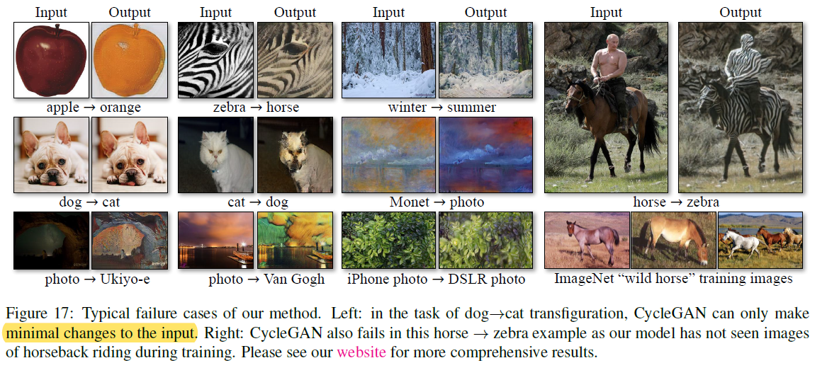
- 얼룩말을 탄 사람 이미지는 없기 때문에 성능이 좋지 않음.
- 모양은 바꿀 수 없음.
'Deep Learning > [논문] Paper Review' 카테고리의 다른 글
| ELMO (0) | 2023.07.06 |
|---|---|
| SegNet (0) | 2023.07.06 |
| XLNet: Generalized Autoregressive Pretraining for Language Understanding (1) | 2023.07.05 |
| Inception-v4, Inception-ResNetand the Impact of Residual Connections on Learning (0) | 2023.07.05 |
| Seq2Seq (0) | 2023.07.05 |


